本笔记直接从 Notion 签出,大部分的 Calculus AB 部分内容没有整理,格式混乱,内容或有错误,仅供参考
本文 All Right Reserved 保留所有权利,禁止商用和任何形式的转载
Unit 1: Limits and Continuity 极限与连续
Limits 极限
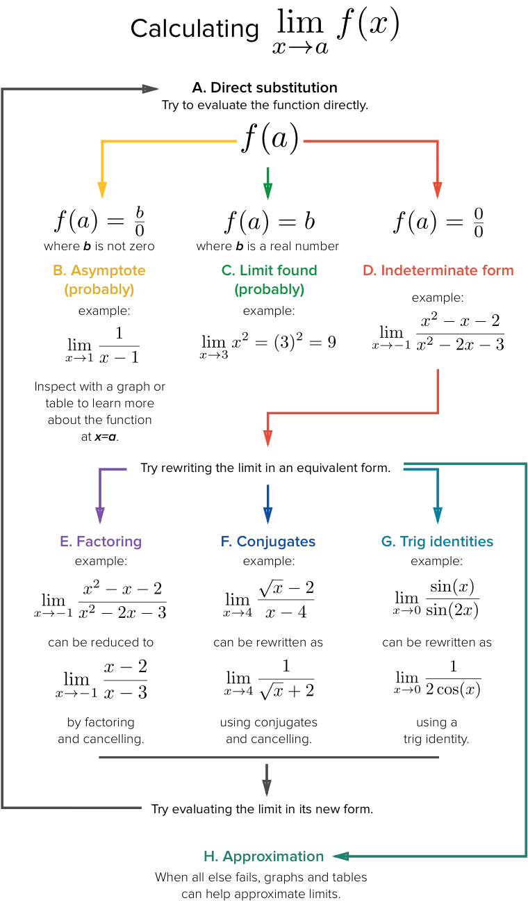
通用分析步骤
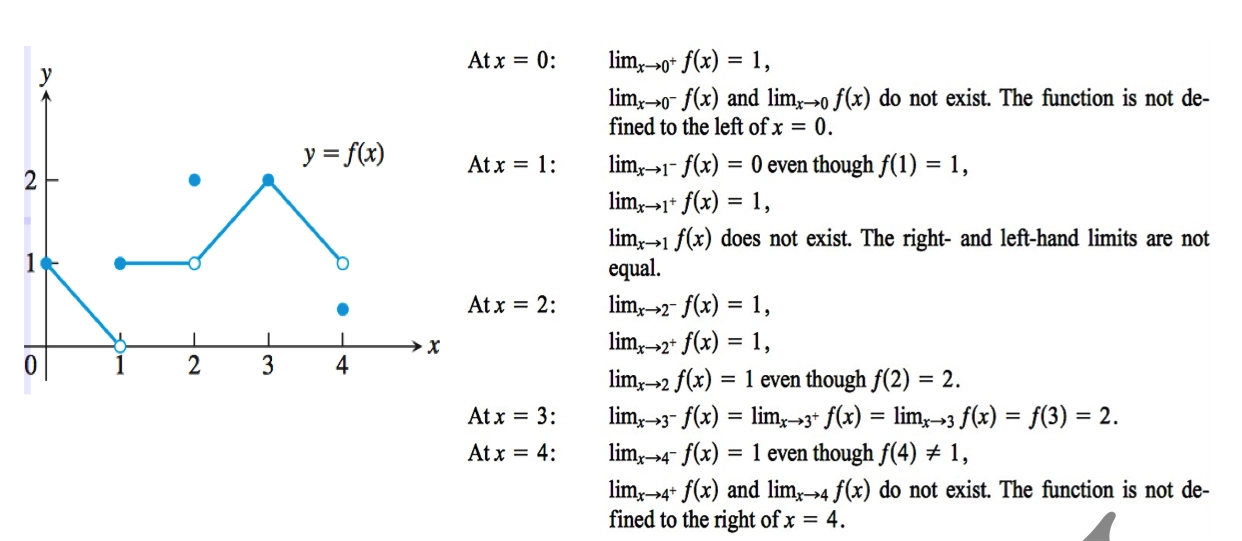
Determine the Existence of Limits 判断极限是否存在
\(1\) 的左极限(即从负方向靠近正方向): \(\lim\limits_{x \to 1^-} f(x)\)
\(1\) 的右极限(即从正方向靠近负方向): \(\lim\limits_{x \to 1^+} f(x)\)
如果左右极限相等,极限存在,反之不存在:\(\lim\limits_{x \to 1^-} f(x) = \lim\limits_{x \to 1^+} f(x) = c\)
例题
Properties of Limits 极限的性质
- 若存在极限 \(\lim\limits_{x \to c} f(x) = L\) 和极限 \(\lim\limits_{x \to c} g(x) = K\),则极限有如下性质
- 数乘法则:\(\lim\limits_{x \to c} [bf(x)] = b \lim\limits_{x \to c} [f(x)] = bL\)
- 加减法则:\(\lim\limits_{x \to c} [f(x)\pm g(x)] = \lim\limits_{x \to c} [f(x)] \pm \lim\limits_{x \to c} [g(x)] = L \pm K\)
- 乘法法则:\(\lim\limits_{x \to c} [f(x)\cdot g(x)] = \lim\limits_{x \to c} [f(x)] \cdot \lim\limits_{x \to c} [g(x)] = L\times K\)
- 除法法则:\(\lim\limits_{x \to c} [\frac{f(x)}{g(x)}] = \frac{\lim\limits_{x \to c} [f(x)]}{\lim\limits_{x \to c} [g(x)]} = \frac{L}{K}, \;\;i.e.\; K \neq 0\)
- 幂法则:\(\lim\limits_{x \to c} [f(x)^n] = \lim\limits_{x \to c} [f(x)]^n = L^n\)
- 极限链式(复合函数)法则:\(\lim\limits_{x \to c} [f(g(x))] = \lim\limits_{u\to\lim\limits_{x\to c}g(x)}f(u)\)
Algebraic Limits 代数极限
- 通常使用因式分解等方法,将原式变换为可以直接带入的极限
Infinite Limits 无穷极限 (BC Only)
- 计算无穷极限时,常考虑为渐近线。
- 对于多项式除法渐近线的判断有如下规则:
- 若存在多项式除法 \(\frac{p(x)}{q(x)}\),其中 \(m\) 为 \(p(x)\) 的最高次项系数,\(n\) 为 \(q(x)\) 的最高此项系数,则有:
\[\begin{cases} m > n & \text{no asymptote} \\ m = n & \text{asymptote: } \frac mn \\ m < n & \text{asymptote: } 0 \end{cases}\]
例题
\(\lim\limits_{x\to-\infty}\frac{-2\sqrt{9x^{10}+2x^8+5}}{-12x^5+4x^3-2x^2-1}=\space?\)
\(\lim\limits_{x\to\infty}\frac{5+e^{-x}}{1-e^{-x}}=\space?\)
\(\lim\limits_{x\to-\infty}\frac{5+e^{-x}}{1-e^{-x}}=\space?\)
If \(f(x) = \begin{cases} \frac{\sqrt{2x+5}-\sqrt{x+7}}{x-2} & x \ne 2 \\ k & x = 2 \end{cases}\), and if \(f(x)\) is continuous a \(x=2\), then \(k=\space?\)
\(f(x)=\frac{x^2+x-20}{x^2-16}\), \(\lim\limits_{x\to-4}f(x)=\space?\)
答案
\(1.\space-\frac12 \\2.\space5 \\ 3.\space-1 \\ 4.\space \frac16 \\ 5.\space -\infty\)
Composite Limits 嵌套极限 (BC Only)
- 若有函数 \(f(g(x))\) 求函数当 \(x \to t\) 时的极限,则有
\[\lim\limits_{x\to t}f(g(x)) = \lim\limits_{y\to\lim\limits_{x\to t}g(x)}f(y)\]
- 嵌套极限中,如果 \(g(x)\) 在趋近过程中是常量,则 \(\lim\limits_{x\to t}f(g(x)) = f(g(t))\)
Squeeze Theorem 夹逼定理 (BC Only)
- 若有函数 \(h(x)\) 定义如下
\[h(x) = \begin{cases}x\sin(\frac1x)&x\ne0\\0&x=0\end{cases}\]
- 函数 \(h(x)\) 满足 \(x \in \mathbb{R}\) 时是否连续?
\[\begin{aligned} & -1\ge \sin(\frac1x)\ge1 \\ \Rightarrow &-|x|\ge x\cdot \sin(\frac1x) \ge -|x| \\ \Rightarrow &\lim_{x\to0}x\cdot \sin(\frac1x) = \lim_{x\to0} |x|=\lim_{x\to0} -|x| = 0 \end{aligned}\]
Continuity 连续
- 如果函数 \(f(x)\)
满足以下三个条件,即称 \(f(x)\) 在
\(x = c\) 处连续
- \(f(c)\) 存在
- \(\lim\limits_{x \to c} f(x)\) 存在
- \(\lim\limits_{x \to c} f(x) = f(c)\)
Continuity on Intervals & IVT 连续与介值定理
Unit 2: Differentiation: Definition and Fundamental Properties 导数的定义与基本性质
Definition of Derivatives 导数的定义
Derivative Rules 求导方法
\(Tangent \space Line: \frac{d(f(x))}{dx} = \frac{P_y-f(x)}{P_x-x}\)
The derivative of an inverse function
Given \(g(x)=f^{-1}(x),\space f(a) = b \space g(b) = a\), than \(g'(b)=\frac1{f'(a)}\)
In general, \(g'[f(x)] = \frac1{f'(x)}\) or \(g'(x) = \frac1{f'(g(x))}\)
particle motion
\[\frac{d}{dx}[\ln(u)] = \frac{u'}{u} \\ u' = u \cdot \frac{d}{dx}[\ln(u)] \\ f'(x) = f(x) \cdot \frac{d}{dx}[\ln(u)]\]
So,
\[\frac d{dx}(x^x)= x^x \cdot \frac d{dx}[x\cdot \ln(x)] \\ = x^x \cdot(1+\ln(x))\]
\[\frac d{dx}[\cos(x)^x], x \in (0, \frac x2) \\ = \cos(x)^x \cdot \frac d{dx}[x\cdot\ln(\cos(x))] \\ = \cos(x)^x \cdot (\ln(\cos(x)) + x\cdot\frac{-\sin(x)}{\cos(x)}) \\ = \cos(x)^x \cdot (\ln(\cos(x)) + x\tan(x))\]
Power Rule 幂法则
Product & Quotient Rules 乘 / 除法则
Differentiability and Continuity 可导与连续
Unit 3: Differentiation: Composite, Implicit and Inverse Functions 复合函数,隐函数,反函数的微分
Chain Rule 链式法则 复合函数求导
Derivatives of Exponential Functions 指数函数的导数
Derivatives of Triangle Functions 三角函数的导数
Derivatives of Log Functions 对数函数的导数
Table of Differentiation Formula 求导公式表
\(\frac d{dx} e^x = e^x\)
\(\frac {d}{dx} a^x = a^x \ln a\)
\(\frac{d}{dx}\ln(u) = \frac{u'}{u}\)
\(\frac d{dx} \log_au= \frac{u'}{u\ln a}\)
\(\frac d{dx}\tan x = \sec^2x\)
\(\frac d{dx} \arctan(u) = \frac{u'}{1+u^2}\)
\(\frac d{dx} \sec x = \sec x \tan x\)
\(\frac d{dx} \arcsin(u) = \frac{u'}{\sqrt{1-u^2}}\)
\(\frac d {dx} \csc x = -\csc x \cot x\)
Implicit Differentiation 隐函数求导
Inverse Function 反函数求导
Higher Order Derivative of a Function 函数的高阶导数
Unit 4: Contextual Application of Derivatives 导数的应用
Interpreting the Meaning of Derivatives 解释导数的含义
L’Hopital’s Rule 洛必达法则
- 若有极限 \(\lim\limits_{x \to n} p(x)\),其中 \(p(x)\) 满足 \(0/0\) 型,或其他形式,则可以通过 \(\text{L'H}\hat o \text{pital's Rule}\) 将原极限转换,使得
\[\lim\limits_{x \to n} [p(x) = \frac{f(x)}{g(x)}] = \lim\limits_{x \to n} \frac{f'(x)}{g'(x)} = \frac{f'(n)}{g'(n)}\]
Unit 5: Analytical Applications of Differentiation 导数的分析及应用
- 直观对于微分中值定理的理解
Mean Value Theorem中值定理
- If \(f\) is continuous on the closed interval and differentiable on the open interval \((a, b)\), then there exists a number \(c\) in \((a,b)\) such that \(f'\left( c\right) =\dfrac{f\left( b\right) -f\left( a\right) }{b-a}\)
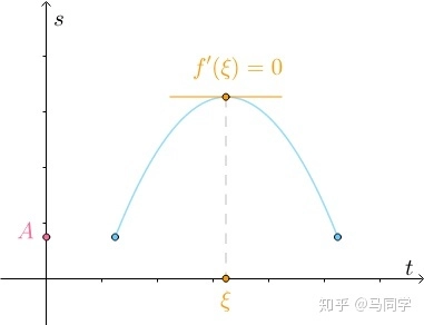
Rolle’s Theorem罗尔定理
- Let \(f\) be continuous on the closed interval \([a,b]\) and differentiable on the open interval \((a, b)\). If\(f(a) = f(b)\), then there is at least one number \(c\) in \((a,b)\) such that \(f'(c) = 0\).
Derivative Test 导数检验
First Derivative Test 一阶导检验
- If \(f'(a) < 0\), then \(f(x)\) is decreasing at \(x = a\)
- If \(f'(a) > 0\), then \(f(x)\) is increasing at \(x = a\)
Second Derivative Test 二阶导检验
- If \(f''(a) > 0\), then \(f(x)\) is concave up at \(x = a\)
- If \(f''(a) < 0\), then \(f(x)\) is concave down at \(x = a\)
- Point of inflection: \(f''(a) = 0\) , must have sign changing.
Critical Point 临界点
- \(f(c)\) is defined at \(c\), also means that \(c \in D_f\)
- \(f'(c) = 0\), or \(f\) is not differentiable at \(f\).
Calculate Critical Point 计算临界点
- Let \(f'(x) = 0\) or \(f'(x) = \text{DNE}\)
Absolute / Relative - Max / Min 极值的理解
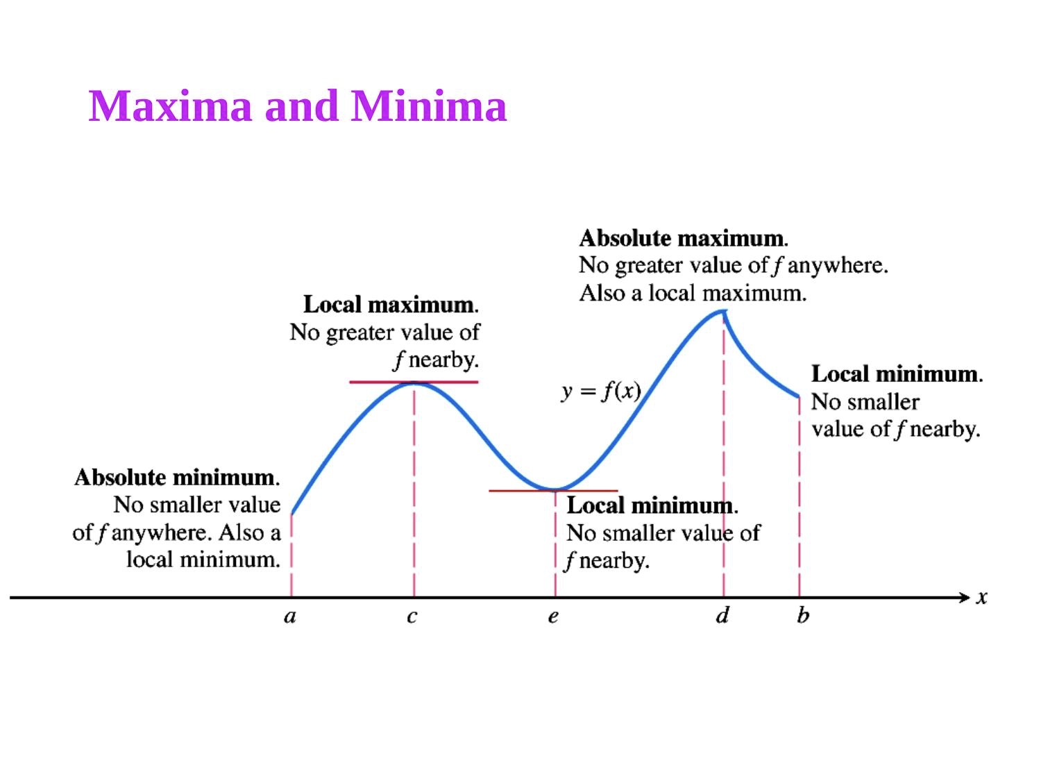
- Absolute Maximum
- Absolute Minimum
- Relative Maximum
- Relative Minimum
Absolute 又名 Global,Relative 又名 Local
Calculate Absolute Maximum / Absolute Minimum 计算绝对最大值和绝对最小值
- 计算出所有临界点并且将端点列入 Candidate Test
- 计算 Candidate Test 中候选点的值
- 对比得到 Maximum / Minimum
Calculate Relative Maximum / Relative Minimum 计算相对最大值和相对最小值
- First Derivative Test 一阶导数判断极值点
- \(f'(x) = 0\) 从正+到负-:Local Minimum
- \(f'(x) = 0\) 从负-到正+:Local Maximum
- \(f'(x) = 0\) 符号不变:无极值
- Second Derivative Test 二阶导数判断极致点
- \(f'(x) = 0\), \(f''(x) < 0\):Maximum
- \(f'(x) = 0\), \(f''(x) > 0\):Minimum
- \(f'(x) = 0\), \(f''(x) = 0\):Test Fail
Linear Approximation 线性估计
- The formula is as follow:
\[dy=f'( x_{0}) \cdot \Delta x \\ y_{1}=y_{0}+dy=f( x_{0}) +f'( x_{0}) \cdot \Delta x( x-a) \]
Optimization Problems 优化问题
通过约束条件和导数值取得最大或最小值,解决优化问题
例 Finding Maximum Volume 寻找最大体积
A manufacturer wants to design an open box having a square base and a surface area of 108 square inches, as shown. What dimensions will produce a box with maximum volume?
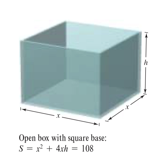
- 列出体积公式:\(V=x^2h\)
- 通过已知的 S 公式得到: \(h=\:\frac{108-x^2}{4x}\)
- 代入体积原公式得到:\(V=x^2(\:\frac{108-x^2}{4x})\)
- 对 \(V=x^2(\:\frac{108-x^2}{4x})\) 求导
- \(V'\)的 Maximum 即为答案
例 Finding minimum distance 寻找最近距离
Which points on the graph of \(y=4-x^2\) are closest to the point \((0,2)\) ?
利用距离公式得:\(d=\sqrt{\left( x-0\right) ^{2}+\left( y-2\right) ^{2}}\)
代入原公式得:\(d=\sqrt{x^{2}+\left( 4-x^{2}-2\right) ^{2}}=\sqrt{x^{4}-3x^{2}+4}\)
对 \(f\left( x\right) =x^{4}-3x^{2}+4\) 求导
令 \(f'(x)=0\),接着利用 First Derivative Test 算出 Maximum, Minimum.
Unit 6: Integration and Accumulation of Chang 积分和累计变化
Riemann Sum 黎曼积分
\[\lim\limits_{n \to +\infty}\sum^n_{i=1}f[a+\frac in(b-a)]\frac{b-a}{n} = \int^a_bf(x)dx\]
The Fundamental Theorem of Calculus and Accumulation Function 微积分基本定理与累积函数
Integrating Using Substitution 换元法积分
Integrating Using Parts 分部积分
Integrating Using Partial Function 部分分式积分
\[d(uv) = udv + vdu \\ \int d(uv) = uv = \int udv + \int vdu \\ \int udv = uv - \int v du\]
Improper Integrals 反常积分
Determine the Improper Integrals 判断反常积分
Determine of Convergence of Improper Integrals 反常积分的敛散性判断
- Comparison Method for Determining of Convergence of Improper Integrals 比较审敛法
- p-Series Method of Determining of Convergence of Improper Integrals 比阶审敛法
Calculation of Improper Integrals 反常积分的计算
Unit 7: Differential Equation 微分方程
- 通过 3Blue1Brown,深入了解微分方程 微分方程 Differential Equation
Solution to the Differential Equation 微分方程的解
Slope Field 斜率场
Application of the Differential Equation 微分方程的应用
Exponential Model 指数模型
一般形式:\(\frac{dy}{dx} = ky\)
- \(k\) 即变化率
对于一阶常微分方程解法
\[\frac{dy}{dx} = ky \\ \frac{dy}{y}=k\cdot dx \\ \ln|y| = kx + C \\ y = e^{kx+C}\]
Logistic Model 人口增长模型
一般形式:\(\frac{dy}{dx} = ky(M-y)\)
- \(k\) 即变化率,\(M\) 为环境最高承载量(即自限函数)
解关于人口增长模型的微分方程
\[\frac{dy}{dx} = ky(M - y) \\ \frac{dy}{y(M-y)} = kdx \\ \int \frac{dy}{y(M-y)} = \int \frac{A}{y} + \frac B{M-y}dy , \frac{A(M-y)+BM}{y(M-y)} \\ A(M-y)+BM=1 \to A=B=\frac 1M \\ \int \frac 1M(\frac1y - \frac1{M-y})dy = \int kdx \\ \ln |M-y| - \ln |y| = -Mkx+C \\ \ln|\frac{M-y}{y}| = -Mkx+C \\ \frac{M-y}{y} = e^{-Mkx+C} \\ \frac My - 1 = e^{-Mkx+C} \\ y = \frac M{1+e^{-Mkx+C}}\]
Euler’s Method 欧拉法
欧拉法本质上是一种折线法,在每次估计后根据步长调整斜率
原理
\[f'(x) \approx \frac{f(x + \Delta x)-f(x)}{\Delta x} \\ f'(x)\Delta x + f(x) \approx f(x + \Delta x)\]
通过 步长 确定 \(\Delta x\), 然后通过导函数 \(f'(x)\) 对原函数 \(f(x)\) 进行估计
每一步估计后需要基于新的导数(变化率)对原函数进行估计
Unit 8: Applications of Integration 积分的应用
Average Value of Function 函数的平均值
Mean Value Theory for Integral 积分中值定理
如果存在 \(f(x)\) 在 \((a, b)\) 范围内连续,则有一点 \(c \in (a, b)\)
\[f_{average}=\frac{\int_a^bf(x)dx}{b-a}=c\]
Motion and Integrals 运动与积分
建议直接查阅 AP Physics C Mech
Area Between Curves 曲线间面积
\[A = \int^b_a[f(x) - g(x)] dx\]
Calculate Volume Using Integrals 用积分计算体积
Disk Model Method 圆盘法
若存在函数 \(f(x)\),则 \(f(x)\) 在区间 \([a, b]\) 绕 \(x\) 轴旋转所形成的体积如下图所示

我们可以将其中 \(\mathrm{d}x\) 旋转的图像视作为以 \(x\) 轴为中心,\(y\) 为半径,\(\mathrm{d}x\) 为高度的圆柱形,而圆柱形体积为 \(V = \pi r^{2} h\),所以我们可以得到
\[\mathrm{d}V = \pi r^{2} h = \pi y^2 \mathrm{d}x = \pi f^2(x)\mathrm{d}x\]
积分后可得
\[\int \mathrm{d}V = V = \pi \int^b_a f^2(x)\mathrm{d}x\]
同理我们可以得到绕 \(y\) 轴旋转所形成的体积为
\[V = \pi \int^b_a(f^{-1}(y))^{2}\mathrm{d}y\]
Washer Method 垫圈法
简而言之,是圆盘法的拓展
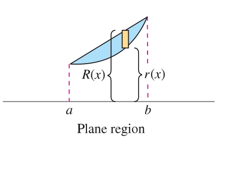
\[V=\pi \int^b_a [R^2(x) - r^2(x)]\mathrm{d}x\]
Shell Model Method 柱壳法 (AP not required)
若存在函数 \(f(x)\),则 \(f(x)\) 在区间 \([a, b]\) 绕 \(y\) 轴旋转所形成的体积如下图所示
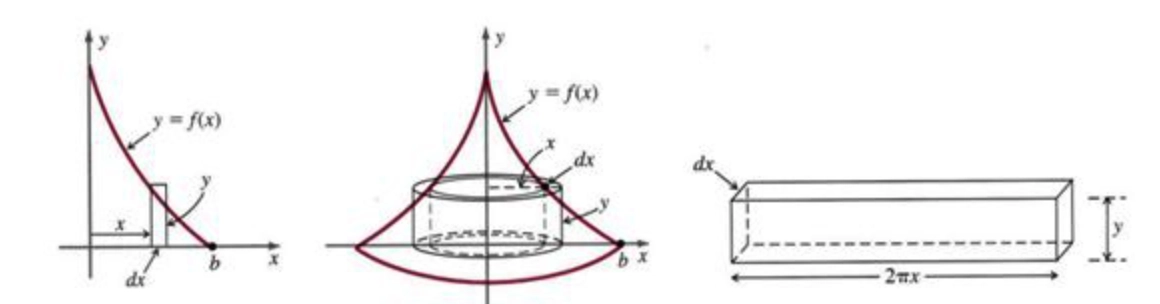
我们可以将其中 \(\mathrm{d}x\) 旋转的图像视作为以 \(y\) 轴为中心,\(x\) 为半径,高度为 \(y\),厚度为 \(\mathrm{d}x\) 的空心圆柱(展开后为长方体),我们知道空心圆柱体公式为 \(V = 2 \pi r \cdot h \cdot w\)
\[\mathrm{d}V = 2 \pi r \cdot h \cdot w = 2\pi x \cdot y \cdot \mathrm{d}x \\[1em] \int^b_a \mathrm{d}V = 2\pi \int^b_a xf(x)\mathrm{d}x\]
同理我们可以得到绕 \(x\) 轴旋转所形成的体积为
\[V = 2\pi \int^b_a yf^{-1}(y)\mathrm{d}y\]
Arc Length 曲线长度
- 推导
\[\begin{aligned} ds &= \sqrt{(dx)^2 + (dy)^2} \\ &= \sqrt{(dx)^2 + (\frac{dy}{dx}\cdot dx)^2} \\ &= \sqrt{(1 + (\frac{dy}{dx})^2)\cdot dx^2} \\ &= \sqrt{1+[f'(x)]^2}\cdot dx \\ \Rightarrow S &= \int^b_a \sqrt{1+[f'(x)]^2}\cdot dx \end{aligned}\]
Unit 9: Parametric Equations, Polar Coordinates, and Vector-Valued Functions 参数方程,极坐标,矢量函数
Parametric Equations 参数方程
- 参数方程便是,\(x\),\(y\),都是关于另一个变量 \(t\) 的函数,例如
\[\begin{cases} x = \cos t \\ y = \sin t \end{cases} \; 0\leq t\leq 2\pi\]
- 这便是一个,单位圆的参数方程,参数方程的定义式如下
\[\begin{cases} x = \phi(t) \\ y = \psi(t) \end{cases}\]
Eliminate the Parameter of Parametric Equation 参数方程的消参
我们通过三角函数恒等式 \(\sin^2\theta + \cos^2\theta = 1\) 可以得到 \(x^2 + y^2 = 1\)
另一个例子
\[\begin{cases} x = 1-t \\ y = \sqrt t \end{cases} \; t \geq 0\]
- 我们可以通过两边同时开方,消掉 \(t\)
\[\begin{aligned} y^2 &= t \\ x &= 1-t = 1-y^2 \\ y^2 &= 1-x \end{aligned}\]
- 对于椭圆方程
\[ \begin{cases} x = a \sin t \\ y = b \cos t \end{cases} \]
- 我们同样的想要得到类似 \(\sin x^{2} + \cos x^{2} = 1\) 的形式,所以我们将其整体平方
\[ \begin{cases} x^{2} = a^{2} \sin^{2} t \\ y^{2} = b^{2} \cos^{2} t \end{cases} \implies \begin{cases} \frac{x^{2}}{a^{2}} = \sin^{2} t \\ \frac{y^{2}}{b^{2}} = \cos^{2} t \end{cases} \]
- 最终得到
\[ \frac{x^{2}}{a^{2}} + \frac{y^{2}}{b^{2}} = 1 \]
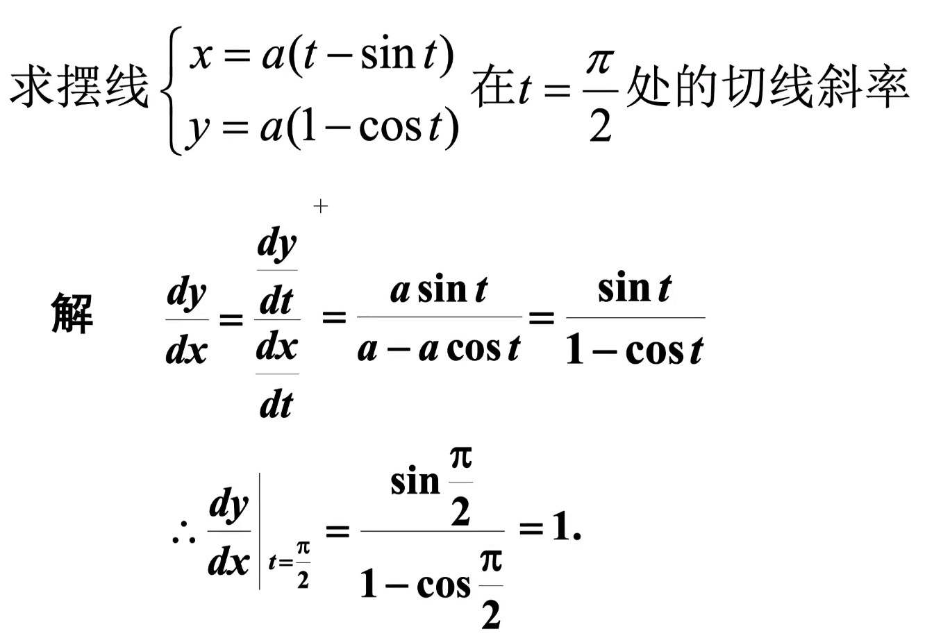
Derivatives of Parametric Equation 参数方程的求导
如果可以消去参数,就是隐函数求导,例如上述例子
- \(y^2 = 1 - x \Rightarrow 2y\cdot y' = -1 \Rightarrow y' = -\frac{1}{2y}\)
如果不可以,则按照导数的定义式推导如下
- 假设我们有以下参数方程
\[\begin{cases} x = \phi(t) \\ y = \psi(t) \end{cases}\]
- 我们可以得到
\[\frac {dy}{dx} = \frac{\frac{dy}{dt}}{\frac{dx}{dt}} = \frac{\psi'(t)}{\phi'(t)}\]
例题
Second Derivatives of Parametric Equation 参数方程的二阶导数
- 根据一阶导数可以推导得到
\[\frac{d^2y}{dx^2} = \frac{d}{dx}(y') = \frac{\frac{dy'}{dt}}{\frac{dx}{dt}} = \frac{\frac{d\frac{\frac{dy}{dt}}{\frac{dx}{dt}}}{dt}}{\frac{dx}{dt}} = \frac{\frac{d(\frac{\psi(t)}{\phi'(t)})}{dt}}{\phi'(t)}\]
例题
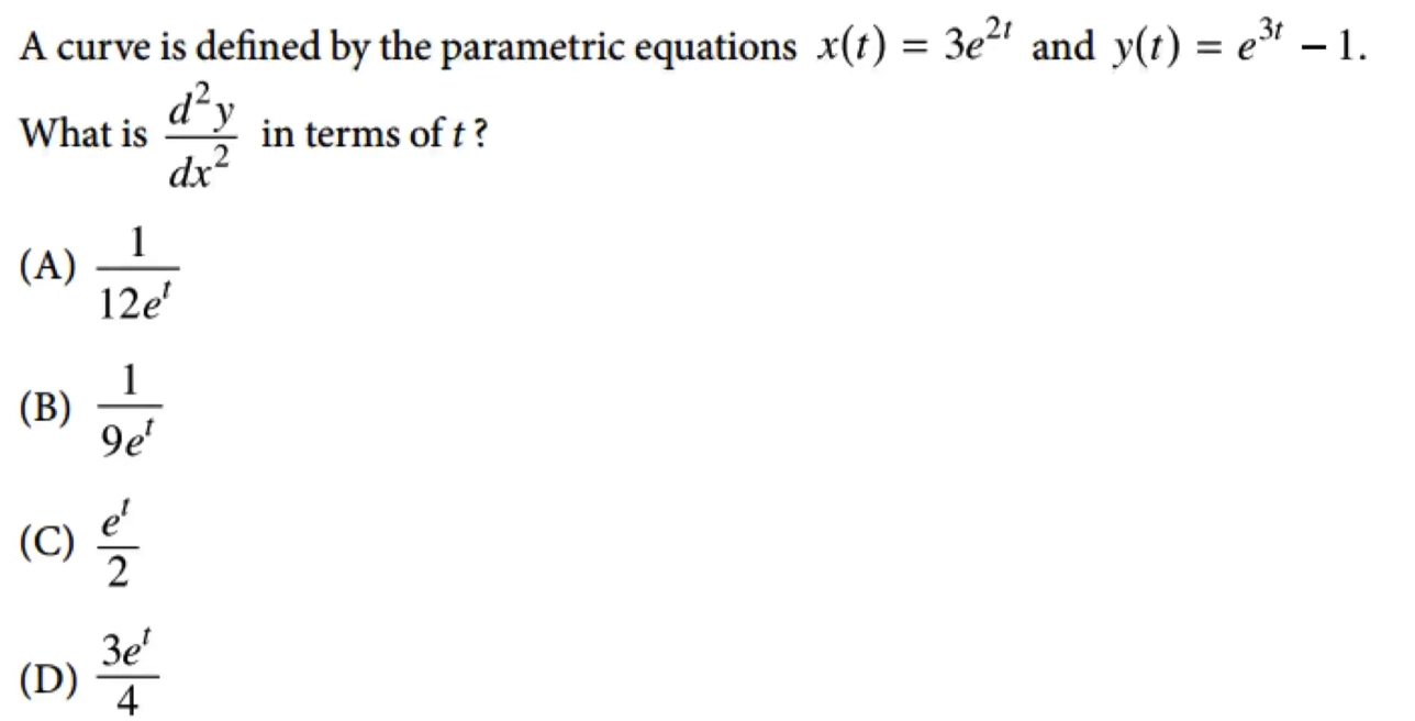
选A
Arc length of Parametric Equation 参数方程的弧长
- 若我们有以下参数方程
\[\begin{cases} x = \phi(t) \\ y = \psi(t) \end{cases}\]
- 其中 \(\phi(t)\),\(\psi(t)\) 在 \([\alpha, \beta]\) 区间中连续且可导
\[\begin{aligned} ds &= \sqrt{(dx)^2 + (dy)^2} \\ &= \sqrt{(\frac{dx}{dt}\cdot dt)^2 + (\frac{dy}{dt}\cdot dt)^2} \\ &=\sqrt{(\phi'(t))^2 + (\psi'(t))^2(dt)^2} \\ &= \sqrt{\phi'^2(t) + \psi'^2(t)}\cdot dt \\ &\Rightarrow S = \int_{t=\alpha}^{t=\beta} \sqrt{(\phi'(t))^2 + (\psi'(t))^2} dt \end{aligned}\]
\[ds=\int^{t=\beta}_{t=\alpha}\sqrt{(\frac{dy}{dx})^2+1}\]
Vector Function 向量函数
对于任意一个向量,在复平面上的表示为:\(\overrightarrow{OA} = \langle a, b \rangle = a\hat i + b\hat j\),例如
- \(\overrightarrow{OA} = \langle 3, 4 \rangle = 3\hat i + 2\hat j\)
对于任意一个向量,我们说向量的模便是向量的长度:\(|\overrightarrow{OA}| = \sqrt{a^2 + b^2}\),例如
- \(\overrightarrow{OA} = \langle 3, 4 \rangle \Rightarrow |\overrightarrow{OA}| = \sqrt{3^2 + 4^2} = 5\)
显然的,我们可以将 \(\overrightarrow{OA} = \langle a, b \rangle = a\hat i + b\hat j\) 表达为一个动态的函数,类似于参数方程
\[\begin{aligned} &\overrightarrow{OA} = \langle f(t), g(t) \rangle = f(t)\hat i + g(t)\hat j \\ &\Rightarrow \begin{cases} x = f(t) \\ y = g(t)\end{cases} \end{aligned}\]
例题
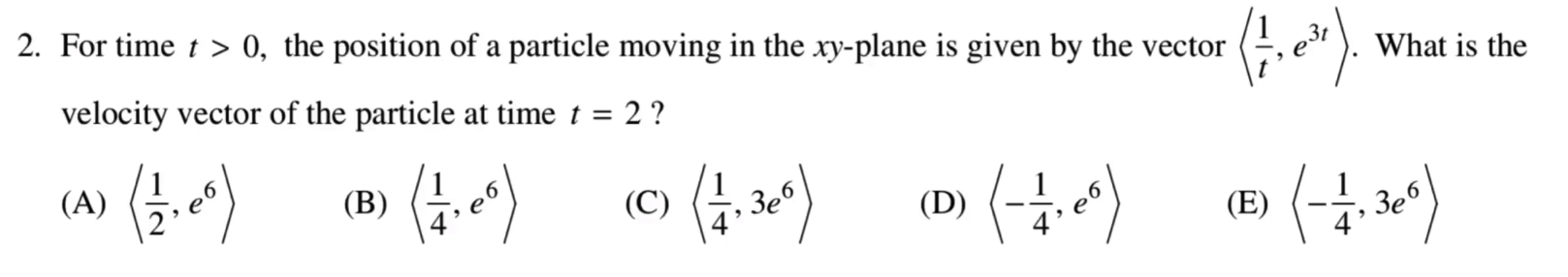
答案选E
Polar Coordinate Function 极坐标函数
Polar Coordinate 极坐标
- 定义
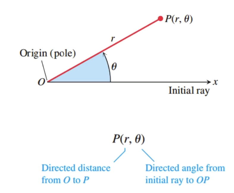
极坐标与直角坐标的转换
- 极转直
\[\begin{cases} x = r\cos \theta \\ y = r \sin \theta \end{cases}\]
- 直转极
\[\begin{cases} r^2 = x^2 + y^2 \\ \tan \theta = \frac{y}{x} \end{cases}\]
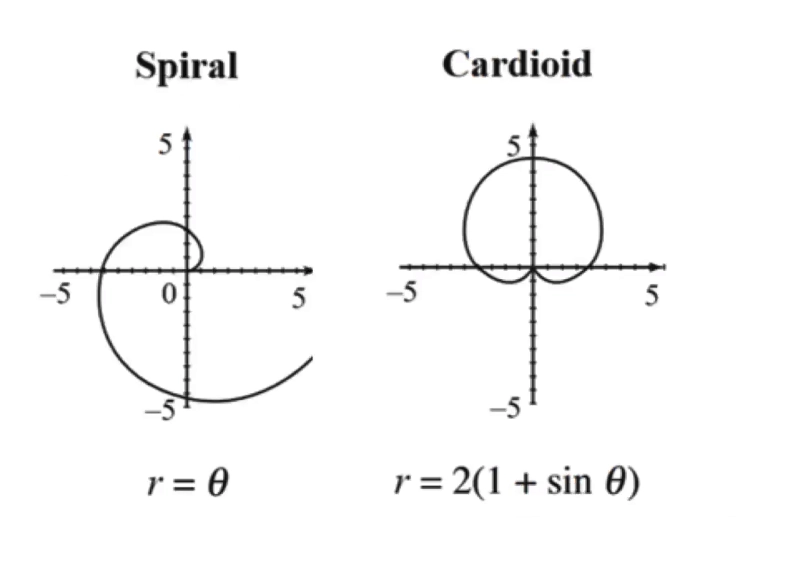
对于常见极坐标图像的理解
- 常用四个点 \(\frac{\pi}{2} \;\; \pi \;\; \frac{3\pi}{2} \;\; 2\pi\) 代入,并给出图像大概的感觉
Circle 圆
计算函数 \(r(\theta) = 2a \cos(\theta)\) 所形成圆的半径 \(r\),和圆心的坐标 \(x, y\)
\[ \begin{aligned} r^{2} &= 2a \cdot (r \cos(\theta)) \\[0.6em] x^{2} + y^{2} &= 2ax \end{aligned} \]
将 \(x^{2} - 2ax\) 配成一个完全平方数,
\[ \begin{aligned} x^{2} - 2ax + a^{2} + y^{2} &= a^{2} \\ (x - a)^{2} + y^{2} &= a^{2} \end{aligned} \]
所以对于函数 \(r(\theta) = 2a \cos(\theta)\) 所形成圆的半径 \(r\),和圆心的坐标 \(x, y\) 分别为 \(r = a, x = a, y = 0\)
同理,对于 \(r(\theta) = 2a \sin(\theta)\) 所形成圆的半径 \(r\),和圆心的坐标 \(x, y\) 分别为 \(r = a, x = 0, y = a\)
Tangent Line 切线
给定点 \(P_{0} = (d, \alpha)\),且点 \(P_{0}\) 是在直线 \(\mathcal{L}\) 上离原点最近的点,求表示 \(\mathcal{L}\) 的极座标函数
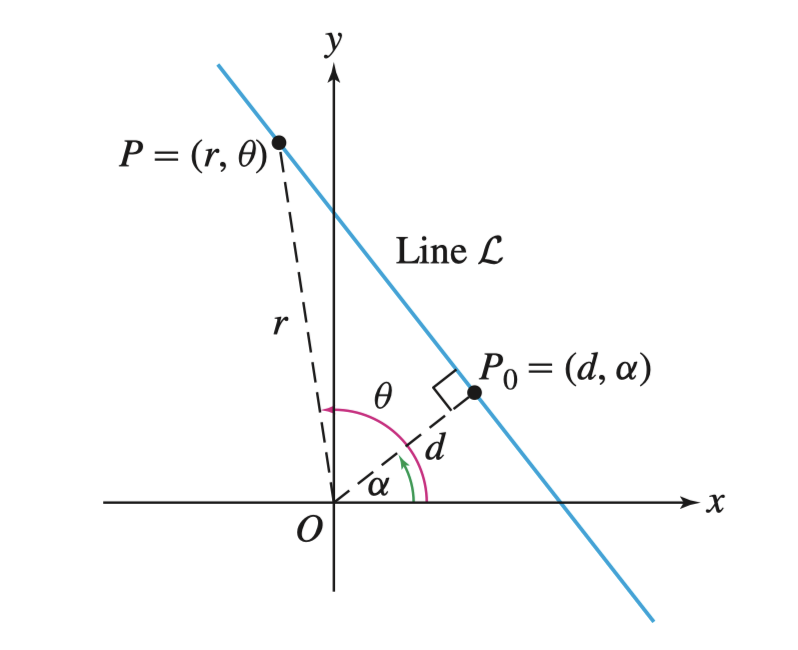
因为 \(P_0\) 在此时为切点,显然 $OP $,所以 \(\triangle OPP_0\) 为直角三角形,所以通过计算 \(\angle POP_{0}\) 的大小(\(\theta - \alpha\))。所以我们知道了边长 \(OP = d\) 和夹角 \(\angle POP_0\),通过三角函数 \(\sec(\theta) = \frac{r}{d}\) 得到 \(r\) 关于 \(\theta\) 的表达式如下
\[ \mathcal{L} : r = d \sec(\theta - \alpha) \]
Line 线
对于任意直线 \(\mathcal{L} : y = mx + b\) 都可以表示为
\[ \mathcal{L} : r = \frac{b}{\sin(\theta) - m\cos(\theta)} \]
若将 \(m\) 拆为 \(m = \frac{k}{q}\),则可表示为
\[ \mathcal{L} : r = \frac{bq}{q\sin(\theta) - k\cos(\theta)} \]
通过下列方式推导
\[ \begin{aligned} \mathcal{L} : y &= \frac{k}{q}x + b \\[0.8em] r \sin(\theta) &= \frac{k}{q} \cdot r \cos(\theta) + b \\[0.8em] r q \sin(\theta) - r k \cos(\theta) &= bq \\[0.8em] \mathcal{L} : r &= \frac{bq}{q \sin(\theta) - k \cos(\theta)} \end{aligned} \]
Derivatives of Polar Coordinate Function 极坐标函数的导数
如果我们有极函数 \(r(\theta)\),所以每个落在函数上点便可表示为 \((r(\theta), \theta)\),然后将极坐标函数转化为参数方程
\[ \begin{cases} x = r(\theta)\cos(\theta) \\ y = r(\theta) \sin(\theta) \end{cases} \]
按照参数方程求导公式 \(\frac {dy}{dx} = \frac{y'(t)}{x'(t)}\) 可
\[ \frac{\mathrm{d}y}{\mathrm{d}x} = \frac{\mathrm{d}(r(\theta)\sin(\theta))}{\mathrm{d}(r(\theta)\cos(\theta))} = \frac{r'(\theta)\sin(\theta) + r(\theta)\cos(\theta)}{r'(\theta)\cos(\theta) - r(\theta)\sin(\theta)} \]
Area of Polar Coordinate Function 极坐标函数的面积
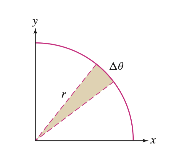
所以我们可以得到极坐标函数的面积
\[ A=\pi r^2\frac{d\theta}{2\pi}=\int_a^b\frac12 r^2(\theta)d\theta \]
Unit 10 Infinite sequences and series 无穷序列
Determine Convergent and Divergent of an Infinite sequence 判断序列敛散性
N-term Test for Divergence N 阶审散法
- 我们存在无限数列单项 \(a_n\),且满足
\[\lim_{n\to \infty}a _n\neq 0 \Rightarrow \sum^{\infty}_{n=1}a_n \; \text{divergent}\]
- N-Term Test 只能测试 发散, 如果不满足本测试, 不能判断数列为 收敛
Integral Test for Convergent 积分判断审敛法
- 积分审敛法的本质仍是 N 阶审散法 和 不定积分中的 p-Series 审敛法
\[\int^{\infty}_1 f(x)dx \Rightarrow \lim_{n\to \infty}a _n\neq 0 \Rightarrow \sum^{\infty}_{n=1}a_n \; \text{divergent} \\ \int^{\infty}_1 f(x)dx \Rightarrow \lim_{n\to \infty}a _n = 0 \Rightarrow \sum^{\infty}_{n=1}a_n \; \text{convergent}\]
Harmonic Series and p-Series 调和级数和 p 级数
- 若存在无限数列
\[\sum_{n=1}^\infty \frac1{n^p}\]
- 如果 \(p>1\) 收敛, \(p\leq1\),发散
- 与不定积分 p-Series 审敛法一致
Direct Comparison Test 直接比较判断敛散
- 若存在两个无限数列
\[S_a = \sum_{n=1}^\infty a_n \;\;\;\;\;\;\;S_b = \sum_{n=1}^\infty b_n\]
- 如果 \(S_a\) 收敛,且 \(S_a > S_b\) 那么显然有 \(S_b\) 收敛
- 如果 \(S_b\) 发散,且 \(S_b > S_a\) 那么显然有 \(S_a\) 发散
- 外敛一定内敛,外散一定内散
- 与不定积分比较审敛法一致
Limit Comparison Test 极限比较审敛法
- 若存在两个级数分别为
\[S_a = \sum_{n=1}^\infty a_n \;\;\;\;\;\;\;S_b = \sum_{n=1}^\infty b_n \\ \lim_{n\to \infty}\frac{S_a}{S_b}>0,\in \mathbb{R}\]
- 那么 \(S_a, \,S_b\) 同时 收敛 或者 发散
Alternative Test 交错级数判别法
- 若存在级数
\[\begin{aligned} &S_a =\sum_{n=1}^\infty(-1)^{n+1}a_n = a_1 - a_2 + a_3 - a_4 + \cdots +(-1)^{n+1}a_n\\ &S_a' = \sum_{n=1}^\infty(-1)^{n}a_n = -a_1 + a_2 - a_3 + a_4 - \cdots + (-1)^{n}a_n \end{aligned}\]
- 就有
\[\lim_{n\to \infty}a_n=0 \;\; \text{and} \;\; a_{n+1} < a_n \Rightarrow S_a \; \text{convergent}\]
只能测试收敛, 如果不满足本测试, 不能判断数列为发散
以 Alternating Harmonic Series 交错调和级数为例
\[\begin{aligned} &S_n = \sum_{n=1}^\infty\frac{(-1)^{n+1}}{n} \\ &\frac{1}{n} > \frac{1}{n+1} \;\; \text{and} \; \lim_{n \to \infty}\frac1n = 0 \\ &\Rightarrow S_n \;\;\text{convergent} \end{aligned}\]
Ratio Test 比值法
- 若存在无限数列
\[\sum^{\infty}_{n=0}a_n = {\displaystyle \sum _{k=0}^{\infty }cr^{k}=c+cr+cr^{2}+cr^{3}+\cdots +cr^k}\]
- 我们能够算出等比数列的公比
\[\frac{a_{n+1}}{a_n}=r\]
- 所以如果有
\[L = \lim_{n\to\infty} \frac{a_{n+1}}{a_n}\]
- 那么便有
\[\begin{cases} L < 1 & \text{convergent} \\ L>1 & \text{divergent}\\ L=1 & \text{pending / test fails} \end{cases}\]
Absolute and Conditional Convergence 绝对收敛和条件收敛
Determine Absolute and Conditional Convergence 判断绝对收敛和条件收敛
- 若存在无限数列
\[S_a = \sum_{n=1}^\infty a_n\]
如果 \(\sum_{n=1}^\infty a_n\) 和 \(\sum_{n=1}^\infty |a_n|\) 均为收敛 则为绝对收敛
如果 \(\sum_{n=1}^\infty a_n\) 收敛和 \(\sum_{n=1}^\infty |a_n|\) 发散 则为条件收敛
以 Alternating Harmonic Series 交错调和级数为例
\[\begin{aligned} &S_n = \sum_{n=1}^\infty\frac{(-1)^{n+1}}{n} \;\; \text{convergent} \\ \text{but} \;\; &S_n' = \sum_{n=1}^\infty|\frac{(-1)^{n+1}}{n}| \;\; \text{divergent} \\ &S_n \;\; \text{contionally convergent} \end{aligned}\]
Absolute and Conditional Convergence in Alternative Series with p-Series Test p 级数检验与交错级数在绝对与条件收敛的关系
- 若存在如下交错级数
\[S_n = \sum_{n=1}^\infty\frac{(-1)^{n+1}}{n^p} = 1 - \frac 1{2^p} + \frac 1{3^p} - \frac 1{4^p} + \cdots, \;\; p > 0 \;\; \lim_{n \to \infty} \frac 1{n^p} = 0\]
- 则有如下结论
\[\begin{cases} p > 1 & \text{Absolute Convergence} \\ 0 < p \leq 1 & \text{Conditional Convergence}\end{cases}\]
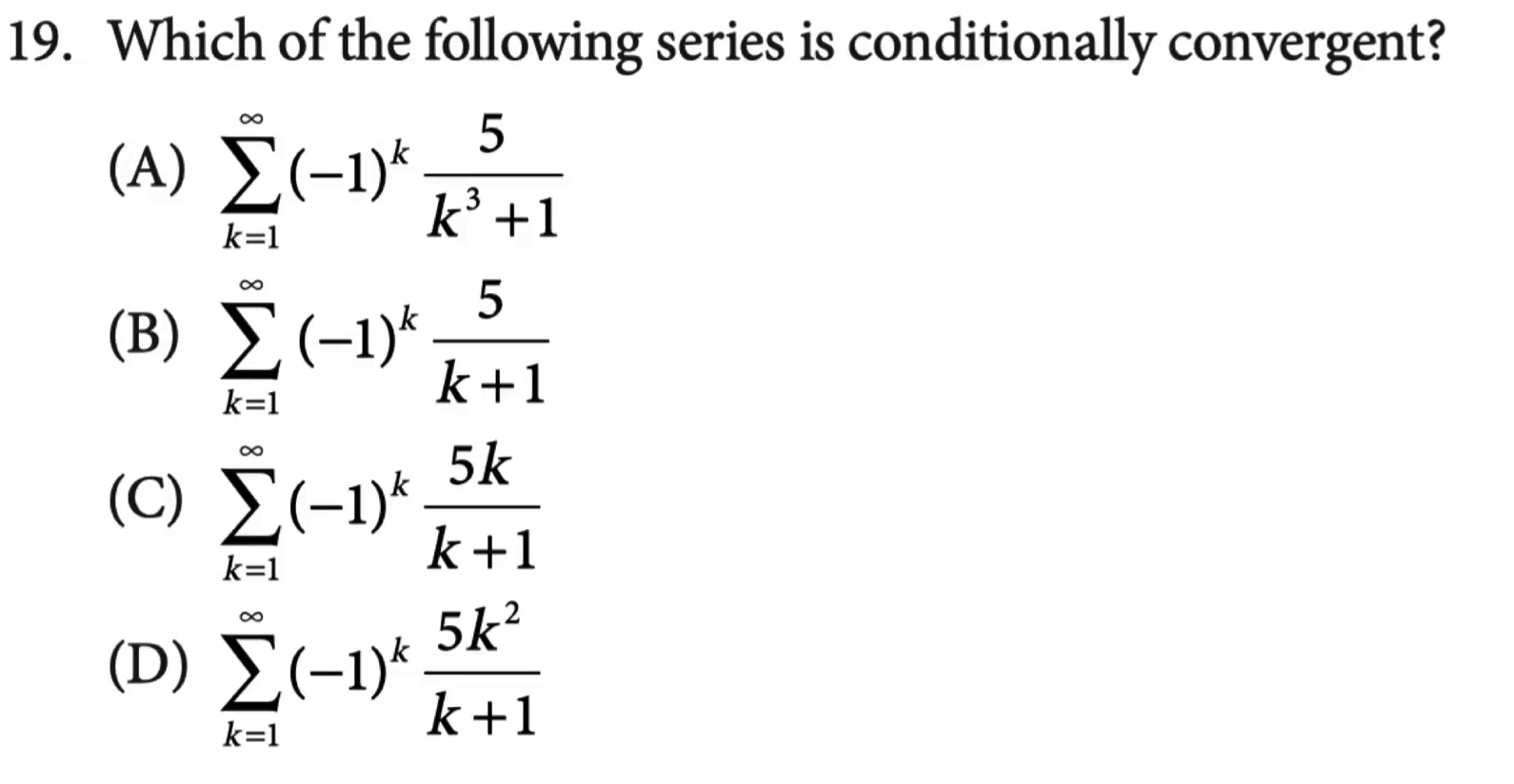
例题
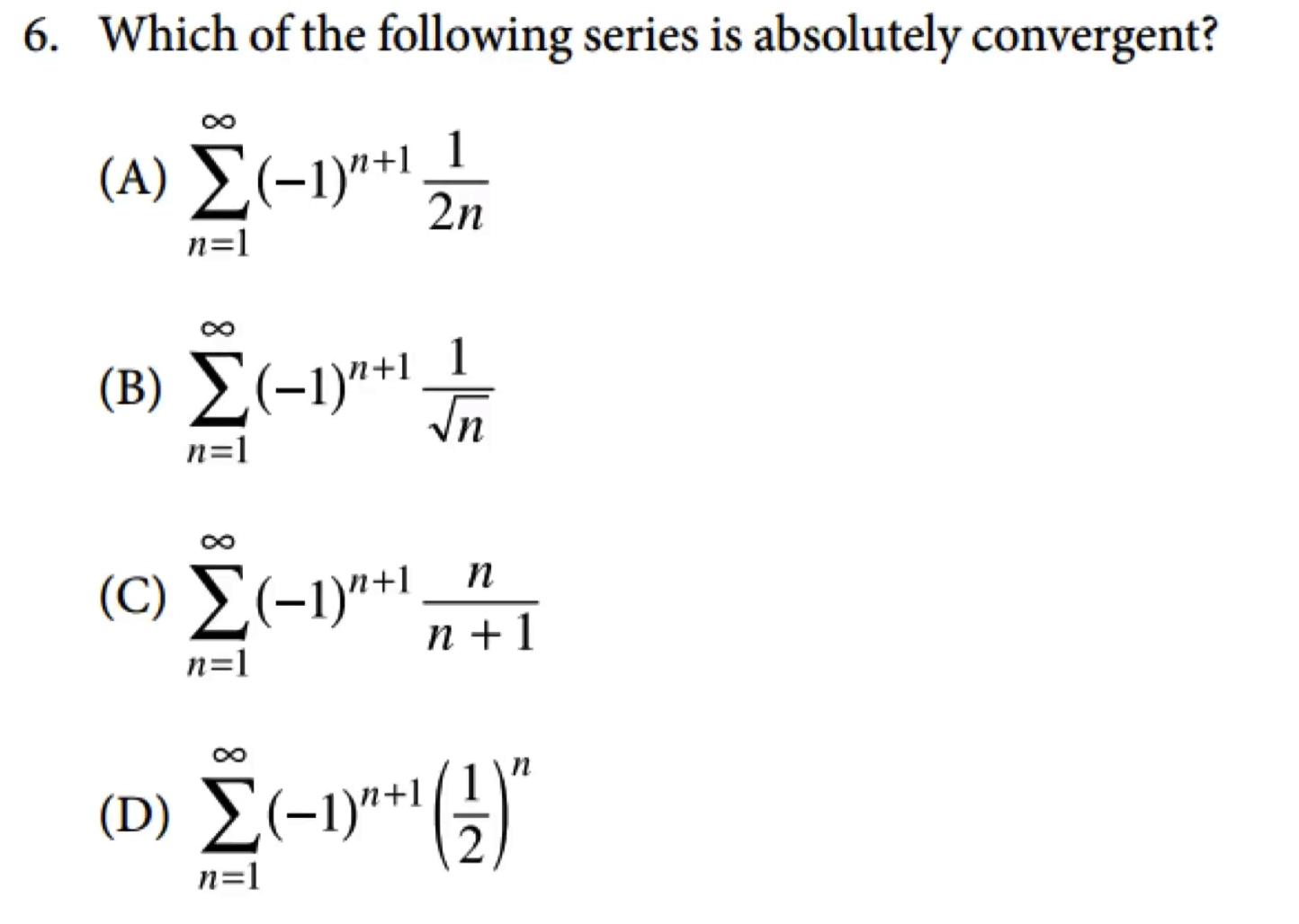
D
B
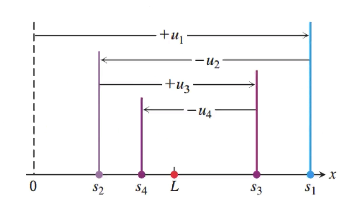
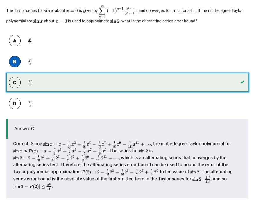
Alternative Series Error Bound Estimate Theorem 交错级数误差界估计定理
- 若存在如下交错级数
\[\sum_{n=1}^\infty(-1)^{n+1}a_n = L\]
- 对于该交错级数的结果有如下结论
\[|S_n - L| \leq |a_{n+1}|\]
- 如下图所示,读者自证不难
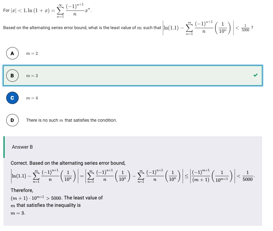
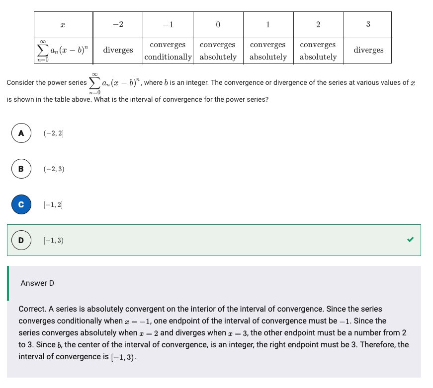
例题
Radius and Interval of Converge of Power Series 幂级数的收敛区间和半径
Power Series 幂级数
- 在 \(x = 0\) 处展开的幂级数为
\[f(x) = \sum^{\infty}_{n=0} c_nx^n = c_0 + c_1x + c_2x^2 + c_3x^3 + \cdots + c_nx^n\]
- 在 \(x = a\) 处展开的幂级数为
\[f(x) = \sum^{\infty}_{n=0} c_n(x-a)^n = c_0 + c_1(x-a) + c_2(x-a)^2 + c_3(x-a)^3 + \cdots + c_n(x-a)^n\]
- 根据 比较审敛法
\[\sum_{n=1}^\infty |a_n| \;\; \text{convergent} \Rightarrow \sum_{n=1}^\infty a_n \;\; \text{convergent}\]
- 所以我们可以通过比值审敛法,通过确定幂级数的绝对值函数收敛,从而确定幂级数收敛
\[\lim_{n\to\infty}|\frac{a_{n+1}}{a_n}\cdot (x-a)| = \lambda \\ \begin{cases} 0 \leq \lambda < 1 & \text{convergent} \\ \lambda > 1 & \text{divergent} \\ \lambda = 1 & \text{pending / test fails} \end{cases}\]
Radius of Converge 收敛半径
- 一般的,幂级数的收敛与否取决于 \(x\) 的范围
\[\lim_{n\to\infty}\left\vert \frac{a_{n+1}}{a_n}\cdot (x-a)z \right\vert < 1\]
- 在这个范围中,幂级数收敛,解得 \(|x-a| < r\),其中 \(r\) 便是收敛半径
Interval of Converge 收敛区间
求出 \(x\) 在收敛半径端点的敛散情况,即可确定收敛区间
例题
For what values of \(x\) do the following series converge?
\[\begin{aligned}&\text{(a)} \;\;\sum_{n=1}^{\infty}(-1)^{n+1} \frac{x^{2 n}}{2 n}=\frac{x^{2}}{2}-\frac{x^{4}}{4}+\frac{x^{6}}{6}-\cdots \\ &\text{(b)} \;\; \sum_{n=0}^{\infty} \frac{(10 x)^{n}}{n !}=1+10 x+\frac{100 x^{2}}{2 !}+\frac{1000 x^{3}}{3 !}+\cdots \end{aligned}\]
\(\text {(a)}\)
\[\begin{aligned} \lim _{n \rightarrow \infty}\left|\frac{u_{n+1}}{u_{n}}\right| &=\lim _{n \rightarrow \infty} \frac{x^{2 n+2}}{2 n+2} \cdot \frac{2 n}{x^{2 n}} \\ &=\lim _{n \rightarrow \infty}\left(\frac{2 n}{2 n+2}\right) x^{2}\\ &=x^2 \end{aligned}\]
- 于是,\(x^2<1\Rightarrow |x|<1\)
- 收敛半径为 \(1\), 接下去判断端点值
- 当 \(x=1\) 时,原级数变为 \(\sum_{n=1}^{\infty}(-1)^{n+1} \frac{1}{2 n}\),根据 交错级数审敛法,级数收敛
- 当 \(x = -1\) 时,原级数变为 \(\sum_{n=1}^{\infty}(-1)^{n+1} \frac{1}{2 n}\),同理收敛
- 所以,收敛区间为 \([-1,1]\)
\(\text{(b)}\)
\[\begin{aligned} \lim _{n \rightarrow \infty}\left|\frac{u_{n+1}}{n_{n}}\right| &=\lim _{n \rightarrow \infty} \frac{|10 x|^{n+1}}{(n+1) !} \cdot \frac{n !}{|10 x|^{n}} \\ &=\lim _{n \rightarrow \infty} \frac{|10 x|}{n+1}=0 \end{aligned}\]
- 所以对于所有 \(x\) ,该级数都收敛
收敛半径的左右端点一定是条件收敛的
Taylor Series 泰勒级数
- 任何函数 \(f(x)\) 都可以被幂级数拟合(从 \(c\) 处展开)
\[f(x) = \sum^{\infty}_{n=0} a_n(x-c)^n\]
- 如何确定 \(a_n\) ? 我们对该幂级数进行多次求导后,观察常数 \(a_n\) 的变化
\[\begin{aligned}f(x) = \sum^{\infty}_{n=0} a_n(x-c)^n &= \textcolor{red}{a_0} + \textcolor{blue}{a_1}(x-c) + a_2(x-c)^2 + a_3(x-c)^3 + \cdots + a_n(x-c)^n \\ f'(x) = (\sum^{\infty}_{n=0} a_n(x-c)^n)' &= \textcolor{blue}{a_1} + \textcolor{green}{2a_2}(x-c) + 3a_3(x-c)^2 + 4a_4(x-c)^3 + \cdots + n \cdot a_n(x-c)^{n-1} \\ f''(x) = (\sum^{\infty}_{n=0} a_n(x-c)^n)'' &= \textcolor{green}{2a_2} + \textcolor{pink}{6a_3}(x-c) + 12a_4(x-c)^2 + 20a_5(x-c)^3\cdots + n (n-1) \cdot a_n(x-c)^{n-1} \\ &\cdots \end{aligned}\]
- 我们通过带入 \(x = c\),便可以确定 \(a_n\)
\[f(c) = a_0 \, , \;\; f'(c) = a_1 \, , \;\; f''(c) = 2a_2 \, , \;\; f'''(c) = 6a_3 \, , \;\; \cdots\, , \;\; f^{(n)}(c) = n!a_n \\ a_n = \frac{f^{(n)}(c)}{n!}\]
- 带回幂级数中我们可以得到一般情况下的泰勒级数(Taylor Series)
\[\begin{aligned} f(x) &= \sum^{\infty}_{n=0} a_n(x-c)^n \\ &= \sum^{\infty}_{n=0} \frac{f^{(n)}(c)}{n!}(x-c)^n \\ &= f(a) + \frac{f'(c)}{1!}\cdot (x-c)+\frac{f''(c)}{2!}(x-c)^2 + \frac{f'''(c)}{3!}(x-c)^3 + \cdots + \frac{f^{(n)}(c)}{n!}(x-c)^n \end{aligned}\]
- 泰勒级数的一般形式
\[f(x) = \sum^{\infty}_{n=0} \frac{f^{(n)}(c)}{n!}(x-c)^n\]
第 \(N\) 阶 (Degree) 的 \(\text{Taylor}\) 多项式,意思是最高次项为 \(N\),但 \(f(a)\)z 算作第 \(1\) 项 (Term)
例题
Maclaurin Series 麦克劳林级数
- \(\text{Maclaurin}\) 级数是 \(\text{Taylor}\) 级数的特殊情况,是函数在 \(x=0\) 处的泰勒展开
\[f(x) = \sum^{\infty}_{n=0} \frac{f^{(n)}(0)}{n!}x^n = f(0) + \frac{f(0)}{1!}x+\frac{f'(0)}{2!}x^2 + \frac{f'(0)}{3!}x^3 + \cdots + \frac{f^{(n)}(0)}{n!}x^n\]
- 一般的,需要记住以下常用函数的 \(\text{Maclaurin}\) 级数
\[\begin{aligned} \frac{1}{1-x}&=1+x+x^{2}+\cdots=\sum_{n=0}^{\infty} x^{n} \quad(|x|<1) \\ \frac{1}{1+x}&=1-x+x^{2}-\cdots=\sum_{n=0}^{\infty}(-1)^{n} x^{n} \quad(|x|<1) \\ e^{x}&=1+x+\frac{x^{2}}{2 !}+\cdots=\sum_{n=0}^{\infty} \frac{x^{n}}{n !} \quad(\text {all real } x) \\ \sin x&=x-\frac{x^{3}}{3 !}+\frac{x^{5}}{5 !}-\cdots=\sum_{n=0}^{\infty}(-1)^{n} \frac{x^{2 n+1}}{(2 n+1) !} \quad(\text {all real } x) \\ \cos x&=1-\frac{x^{2}}{2 !}+\frac{x^{4}}{4 !}-\cdots=\sum_{n=0}^{\infty}(-1)^{n} \frac{x^{2 n}}{(2 n) !} \quad(\text {all real } x) \\ \ln (1+x)&=x-\frac{x^{2}}{2}+\frac{x^{3}}{3}-\cdots=\sum_{x=1}^{\infty}(-1)^{n-1} \frac{x^{n}}{n} \quad(-1<x \leq 1) \\ (1+x)^{p}&=\sum_{k=0}^{\infty} \frac{p(p-1) \ldots (p-k+1)}{k !} x^{k}, |x|<1, p\in \mathbb{R}\end{aligned}\]
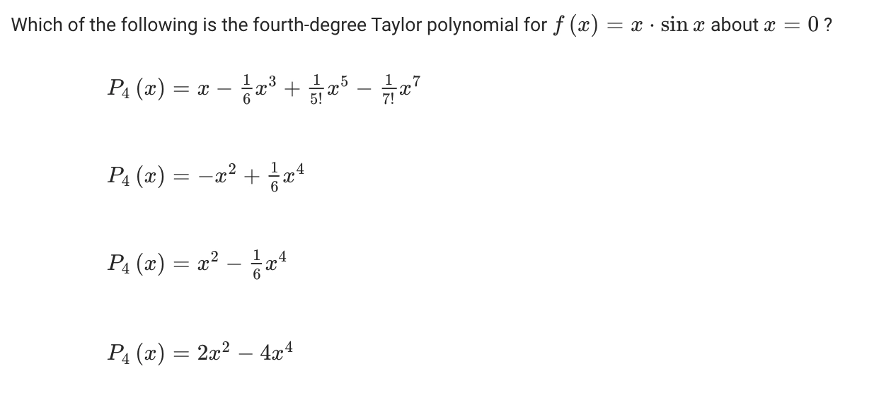
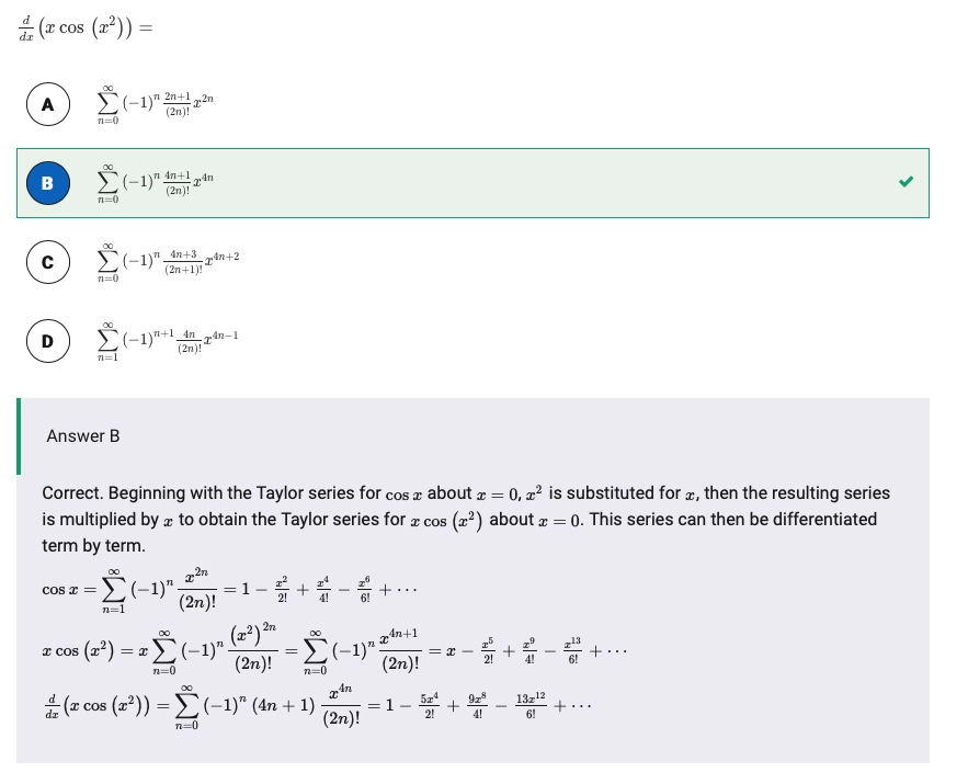
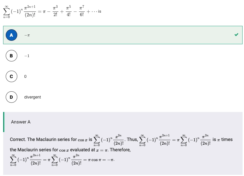
例题
Let \(f\) be a function such that \(f'(x) = \sin (x^2)\) and \(f(0)=0\). What are the first nonzero terms of the Maclaurin series or \(f\)?
\[P_3(x) = \frac{x^3}{3} - \frac{x^7}{42}+\frac{x^{11}}{1320}\]
A function \(f\) has a Maclaurin series given by \(2+3x+x^2+\frac 13 x^3 + \cdots\) , and the Maclaurin series converges to \(f(x)\) for all real numbers \(x\), If \(g\) is the function defined by \(g(x) = e^{f(x)}\), what is the coefficient of \(x^2\) in the Maclaurin series for \(g\)?
\[ \begin{aligned} g(x) &\approx g(0) + \frac{g'(0)}{1!}x +\frac{g''(0)}{2!}x^2 \\[0.6em] g''(0) &= e^{f(0)}\cdot f'(0) + e^{f(0)}\cdot f'^2(0) = 3e^2 + 9e^2 = 11e^2 \\[0.6em] \frac{g''(0)}{2!} &= \frac {11e^2}{2} \end{aligned} \]
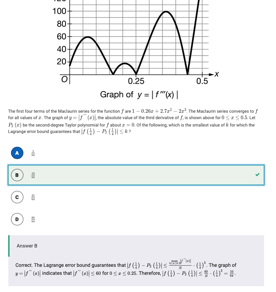
Taylor Polynomial Reminder and Lagrange Error Bound 泰勒多项式余项与拉格朗日误差
Taylor Polynomial Reminder 泰勒多项式余项
- 我们对函数 \(f(x)\) 在 \(a\) 泰勒展开所得到的泰勒级数如下
\[f(x) = \sum^{\infty}_{n=0} \frac{f^{(n)}(a)}{n!}(x-a)^n\]
- 对于无限项的泰勒级数而言,可以完全等价于函数 \(f(x)\),但通常在实际情况下,我们不会求解泰勒级数的无穷项,一般是 \(k\) 个有限项,所以我们有泰勒多项式(Taylor Polynomial),所以此时 \(f(x)\) 与泰勒多项式的关系是约等于
\[f(x) \approx \sum^{k}_{n=0} \frac{f^{(n)}(a)}{n!}(x-a)^n=f(a) + \frac{f'(a)}{1!}\cdot (x-a)+\frac{f''(a)}{2!}(x-a)^2 + \frac{f'''(a)}{3!}(x-a)^3 + \cdots + \frac{f^{(k)}(a)}{k!}(x-a)^k \]
- 所以对于一个有限项的泰勒多项式而言,相对于原函数一定存在差别,而这个差别便是泰勒多项式余项 \(R_k(x)\)(Taylor Polynomial Reminder)
\[f(x) = \sum^{k}_{n=0} \frac{f^{(n)}(a)}{n!}(x-a)^n=f(a) + \frac{f'(a)}{1!}\cdot (x-a)+\frac{f''(a)}{2!}(x-a)^2 + \cdots + \frac{f^{(k)}(a)}{k!}(x-a)^k + R_k(x)\]
- 而 \(R_k(x)\) 的表达式便是拉格朗日余项
\[R_k(x) = \frac{f^{(k+1)}(\xi)}{(k+1)!}(x-c)^{k+1}, \;\; c < \xi < x\]
拉格朗日余项公式的推导
- 我们有拉格朗日中值定理,如下
\[f'(c) = \frac{f(b) - f(a)}{b - a}, \;\; c\in(a, b)\]
- 即函数上一定存在一个当 \(x= c\) 时的瞬时变化率,可以刚好等于函数平均变化率的点
- 推广在参数方城下得到柯西中值定理,即
\[\frac{g'(\xi)}{h'(\xi)} = \frac{g(b) - g(a)}{h(b)-h(a)}\]
- 重新观察余项
\[R_k(x) = \frac{f^{(k+1)}(a)}{(k+1)!}(x-a)^{k+1} + \frac{f^{(k+2)}(a)}{(k+2)!}(x-a)^{k+2} + \cdots + \frac{f^{(n+1)}(a)}{(n+1)!}(x-a)^{n+1}\]
- 可以发现 \((x-a)^{k+1}\) 为余项通项,可以提出。为了简单计算,我们定义函数 \(S_k(x)\) 如下
\[S_k(x) = (x-a)^{k+1}\]
- 计算提取后的结果后还是很复杂,发现 \(R_k(0) = 0\),\(S_k(0) = 0\),便进行如下变换
\[\frac{R_k(x)}{S_k(x)} = \frac{R_k(x)-0}{S_k(x)-0} = \frac{R_k(x) - R_k(0)}{S_k(x) - S_k(0)}\]
- 不难发现最后的式子与柯西中值定理神似,同理继续变换
\[\frac{R_k(x) - R_k(0)}{S_k(x) - S_k(0)} = \frac{R_k'(\xi_1) - 0}{S'_k(\xi_1) - 0} = \frac{R_k'(\xi_1) - R'_k(0)}{S'_k(\xi_1) - R'_k(0)} = \frac{R''_k(\xi_2)}{S''_k(\xi_2)} = \ldots \]
- 我们可以发现可以一直变换下去,直到 \(k+1\) 次导 \(S_k(x)\) 不可继续再导,便可以得到如下推导
\[\frac{R_k(x)}{S_k(x)} = \frac{R'_k(\xi_1)}{S'_k(\xi_1)} = \frac{R''_k(\xi_2)}{S''_k(\xi_2)} = \ldots = \frac{R^{(k+1)}(\xi_{k+1})}{(k+1)!}\]
- 而我们显然需要将 \(R_k(x)\) 的计算脱离 \(R_k(x)\) 导数及其本身,要引入原式 \(f(x)\) 的计算,所以要将 \(R^{(k+1)}(\xi_{k+1})\) 变化为 \(f(x)\) 的形式,可以先得到如下结论
\[P(x) = \sum^{k}_{n=0} \frac{f^{(n)}(a)}{n!}(x-a)^n=f(a) + \frac{f(a)}{1!}\cdot (x-a)+\frac{f'(a)}{2!}(x-a)^2 + \frac{f'(a)}{3!}(x-a)^3 + \cdots + \frac{f^{(k)}(a)}{k!}(x-a)^k\\[0.3em] f(x) = P(x) + R_k(x) \Leftrightarrow R_k(x) = f(x) - P(x) \\[0.8em] R^{(k+1)}(\xi_{k+1}) = f^{k+1}(\xi_{k+1})\]
- 所以最后我们可以整理得到,拉格朗日余项
\[R_k(x) = \frac{f^{(k+1)}(\xi)}{(k+1)!}(x-a)^{k+1}\]
一般的,我们无法确切的知道 \(\xi\) 的具体位置,所以只能估计拉格朗日余项的最大值 \(f^{(k+1)}(x) \leq \max |f^{(k+1)}(\xi)|\)
\[|R_k(x)| \leq \max \bigg|\frac{f^{(k+1)}(\xi)}{(k+1)!}(x-c)^{k+1}\bigg|\]
例题