本笔记直接从 Notion 签出，格式混乱，内容或有错误，仅供参考
本文 All Right Reserved 保留所有权利，禁止商用和任何形式的转载!

AP 各学科「速成」笔记导览

Unit 1: Exploring One-Variable Data 单变量数据探索

Intro Terms 术语介绍

• Individual: Object described by data 研究对象
• Variable: Characteristic of an individual (varies across individuals) 研究对象的特征（变量）
• Observation: The value of a variable for an element (also called measurement) 数据
• Data Set: A collection of observations of one or more variables 数据集
• Categorical / Qualitative Data: Places an individual into one of several groups or categories 定性数据（分类数据）
  • 分类数据加减乘除没有意义
• Quantitative Data: Places an individual on a scale that represents an amount of something 定量数据
  • Discrete Data: Only certain values exist (usually integers) 离散数据
    • 例如，人数，鞋码（虽然有 38.5 这种鞋码），但只有特定的数值可以取
  • Continuous Data: All real numbers are possible (maybe with some limitations, such as no negative numbers) 连续数据，所有的实数都可以取
    
• Univariate Data: One Variable 单元数据
• Bivariate Data: Two Variables 二元数据
• Multivariate Data: More than two variables 多元数据

Univariate Categorical Data 单元定性数据

• 假设你在调查某课堂中学生的国籍，数据如下

England Italy USA USA USA USA USA USA USA USA USA USA USA USA USA USA USA USA USA USA USA

• 我们便可以得到下面两张图，第一张为频数表（Frequency Table），第二张为条形图（Bar Graph）

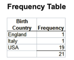
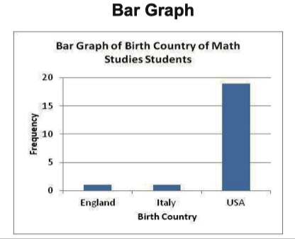
• 频数便是该类变量在数据中出现的次数，条形图则是依据频数表绘制的
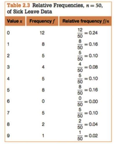
• 如果我们要获得每个类型在数据中的占比，则可以使用 相对频数表（Relative Frequency Table）

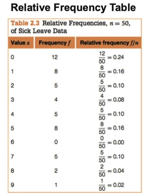
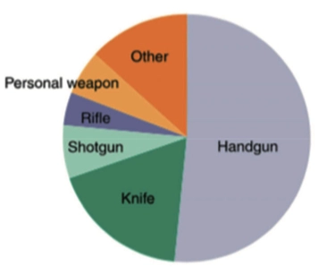
• 通过 相对频数表，我们就可以得到占比及上图中的 饼图（Pie Graph）

Univariate Discrete Quantitative Data 单元离散定量数据

• 同理，见上，几乎没有区别

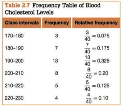
Univariate Continuous Quantitative Data 单元连续定量数据

• 对于像是这样的连续数据

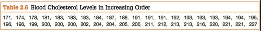
• 简单的频数分析已经失去了意义，因为重复次数基本不多
• 所以我们需要人为分组，将其划分成几个区间

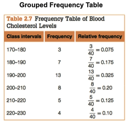
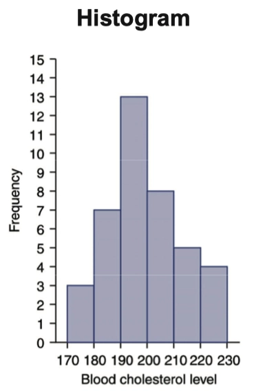
• 哦片；通过分组后计算得到的 分组频数表（Grouped Frequency Table），可以绘制成直方图（Histogram）

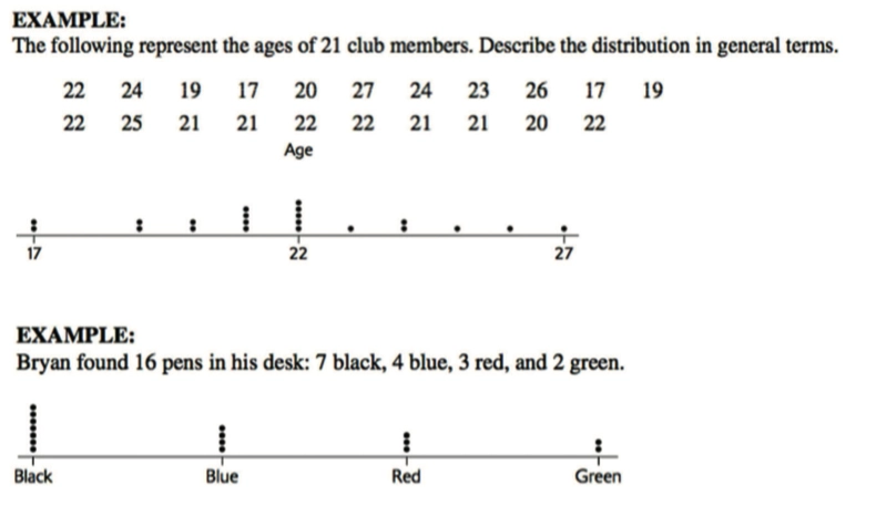
Dot plots 点状图

• 点状图通常用于描述那些变量类型比较少的定性数据和离散数据

Stemplots 茎叶图

• 茎叶图通常用来分组定量的离散数据

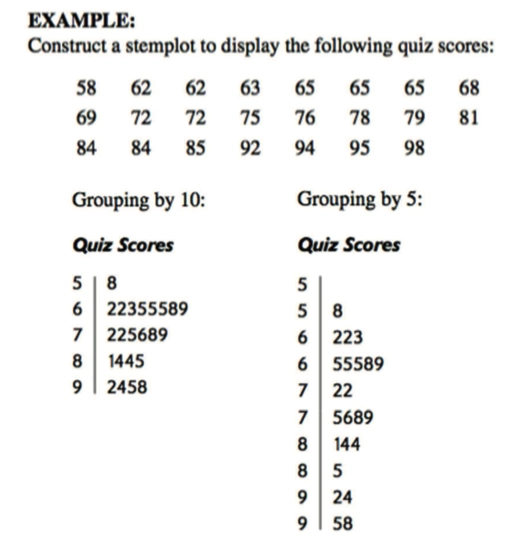
如图中将 5，6，7 等作为茎，然后将属于该茎的另一些字符填入便完成了茎叶图

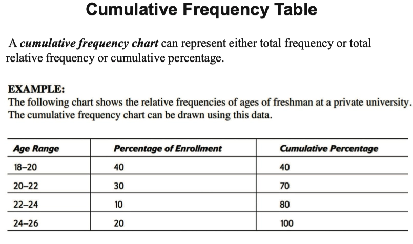
Cumulative Frequency Table 累计频数表

• 累计频数表一般用于总频率或总相对频率或累积百分比。

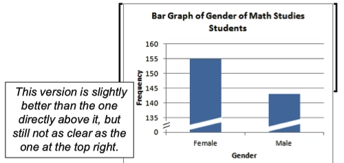
Bad Graph 分辨错误的图表

• 如下图中，左图中的数值差异过于明显，标尺存在错误，不能从 0 直接到 140，而右图是相对合理的

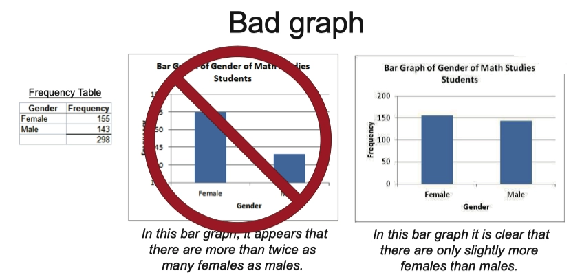
• 但下图中这样的形式也是可以的，通过标记的方式可以让标尺从 0 直接到 135

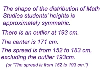
Interpretation of Graph 对图像的解释

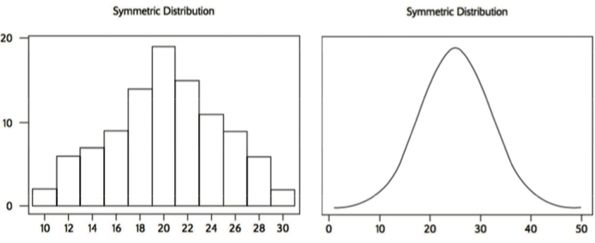
• Shape: symmetric, skewed to left, skewed to right (cluster and gap) 形状
• Outliers: values separated from other values 离群值
• Center: about half of values below & half above 中心
• Spread: specify smallest to largest values 范围
• In context: 联系上下文，加上单位等
• 可以简记为 SOCS

Graph Shape 图像形状

• Symmetric Distribution 对称分布

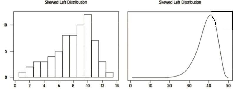
• Skewed Left Distribution 左偏分布
  • 需要注意的是，左偏分布实际上图像是向右偏的，这是因为 Skewed 翻译过来的意思叫作偏离，而不是偏向，偏离左边的分布自然就是偏向右边的分布

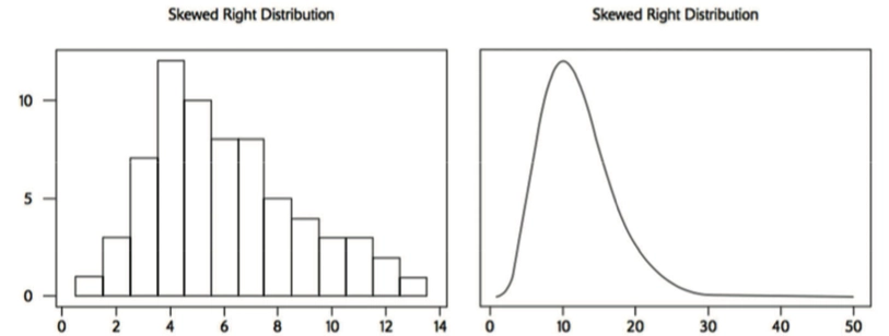
• Skewed Right Distribution 右偏分布

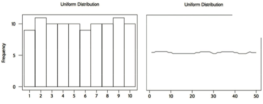
• Uniform Distribution 均匀分布

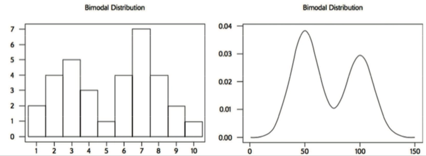
• Bimodal Distribution 双峰分布

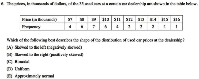
• Practice: B

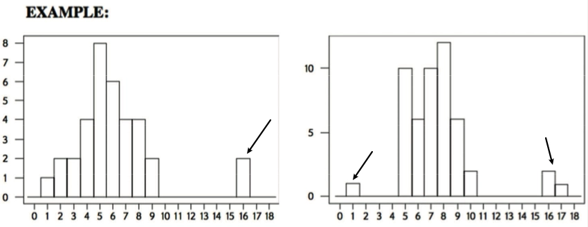
Outliers 离群值

• 如下图所示，离中心离的远，便为离群值

Center and Spread 中心和范围

• Center 数据的中心值一般取中位数
• Spread 数据的范围一般取极差

Interpretation of Stemplots or Histogram

• 通过 SOCS 这四个方面来解释图表

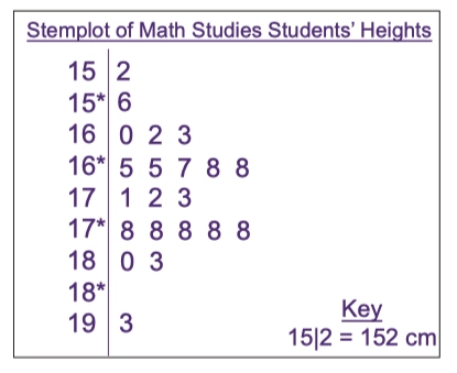
注意：在 Stemplots 中 必须要写形如这样的 Key 否则将会被扣分

Measure of Center 中心的计算

Measure of Mode 众数的计算

• Mode 众数，出现频数最多的数字

• Group Frequency Table 中便无法找到众数

Measure of Median 中位数的计算

• Median 中位数，出现在数据中间的数字
• 计算方式：样本大小为 \(n\) ，若 \(n\) 为偶数，中位数便是 \(\frac n2\) 与 \(\frac n2 +1\) 位置上两个数字的平均值，若 \(n\) 为奇数，中位数便是 \(\frac {n+1}2\)

Measure of Mean 平均数的计算

• Mean 平均数，所有数据的算数平均数
  • 计算方法： \(\bar x = \frac 1n \cdot \sum^n_{i=0} x_i\) ，加权平均数： \(\bar x = \frac 1n\cdot\sum^n_{i=0} x_i \cdot f(x_i)\)

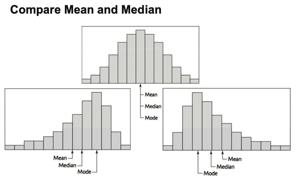
Compare Mean and Median 对比中位数与平均数

• The median is a resistant measure of center because it is relatively unaffected by extreme observations. The mean is nonresistant.
• 中位数是有抗性的，而平均数对于离群值是没有抗性的，容易被离群值带偏

Median and Quartiles 中位数与四分位数

• Lower Quartile, First Quartile, \(Q_1\) 25% of observations are less than this value，前 25% 的数据分界线
• Middle Quartile, Median, Md, \(Q_2\) 50% of observations are less than this value，前 50% 的数据分界线（中位数）
• Upper Quartile, Third Quartile, \(Q_3\) 75% of observations are less than this value，前 75% 的数据分界线

\[Q_1: \frac{1 \times (n + 1)}{4}\;,\; Q_2: \frac{2 \times (n+1)}{4} = \frac{n+1}{2}\;,\;Q_3: \frac{3\times(n+1)}{4}\]

• \(Q_1\) 和 \(Q_3\) 的位数计算需要四舍五入

Measure of Spread (Dispersion) 数据范围的衡量

• Range 极差: \(\text{Max - Min}\)
• Interquartile Range（IQR）分位数范围：\(Q_3 - Q_1\)
• Standard Deviation 标准差 \(s_x\)

\[s_x = \sqrt{\frac 1{n-1}\cdot \sum^n_{i=0}(x_i-\bar x)^2} = \sqrt{\frac {\text{SST}}{n-1}}\]

Differentiation of Notation for Different Scope 不同语境下的符号分别

• 一般的，统计学习是通过样本估计总体，所以对于样本和总体，有不同的统计量符号用以区分 > 进一步而言，因为通常在现实情况下我们没法准确的估计总体，所以 \(\mu \neq \overline{x}\) 这种符号的区分是很有必要的

\[ \begin{aligned} &\text{Population} & \text {Sample} \\ \text{mean}~~~~~~&\mu &\bar x \\ \text{variance}~~~~~~&\sigma ^ 2&s^2 \\ \text{standard deviation}~~~~~~&\sigma & s \\ \text{proportion}~~~~~~&p & \hat p \end{aligned} \]

Standard Deviation 标准差

• The standard deviation \(s_x\) measures the typical distance of the values in a distribution from the mean.

  • If standard deviation is low, this indicates observation of data points tend to be close to the mean
  • If standard deviation is high, this indicates observation of data points are spread out

• Variance \(s_x^2 = \frac1{n-1}\cdot\sum^n_{i=0}(x_i - \bar x)^2 = \frac{\text{SST}}{n-1}\)

• Example

  

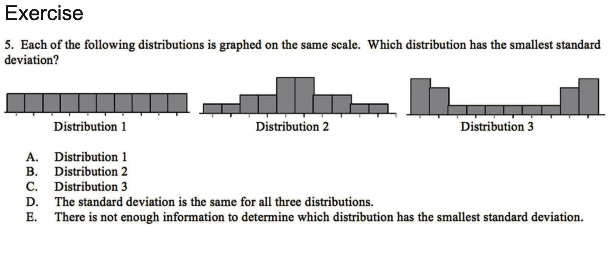
  • 2 < 1 < 3 选 B

1.12.1 Compare the Resistance of Different Types of Spreads 比较不同种类数据范围之间对离群值的抗性

• 对于 极差 来说，离群值显然是会对其数值造成很大的影响
• 而对于 标准差 来说，其引入了平均值和对具体值对计算，同样会受到离群值较大的影响
• 所以 IQR 同样具有 Median 的特性，即只关心数位不关心具体数值，这样可以很好的保证其不受到离群值的影响，所以 IQR 同样具有 Resistance 离群值抗性

1.12.2 Identifying Outliers by 1.5 IQR Rule 通过 1.5 IQR 法则确定离群值

• Interquartile range: \(Q_3 - Q_1\)
• Upper boundary of outliers: \(Q_1 - 1.5\times(\text{IQR}))\)
• Lower boundary of outliers: \(Q_3 +1.5\times (\text{IQR})\)

Only FRQ doesn’t need to exactly calculate and identify the outliers by 1.5 IQR rule. All the problems in MCQ which are related with outliers must be exactly calculate with IQR.

1.13 Measures of Position 位置的衡量

• Percentile is a measure of position, which is represented observation at \(k\%\) positions.
• e.g. the value at \(40\%\) positions

\[l_k = \frac k{100} \times (n+1)\]

1.13 Z-scores 标准化

• Z-scores standardization is a meaningless value unless you compare it with other Z-scores. Z-scores could regularize all the observations of data set into one universal standard, so-called “standardization”. It is equivalent that you measure the distance between the observation and mean by standard deviation \(\sigma\) just like a unit.

\[z=\frac{x - \mu}{\sigma}\]

• Example

  Jenny earned a score of 87 on her statistics test. The class mean was 80 and the standard deviation was 6.1. She earned a score of 82 on her chemistry test. The chemistry scores had a mean of 76 and standard deviation of 3.2. On which test did Jenny perform better relative to the rest of her class?

  Chemistry

1.14 Boxplot Graph 箱型图

• Boxplot graph contains following several information:
  • Min - Q1 - Median - Q3 - Max

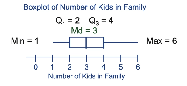
• In general, outliers are represented by notations such that *, -, +, etc

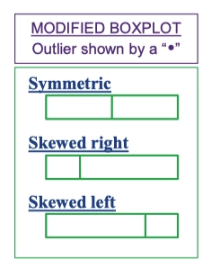
• Differentiated median line of boxplot graph could represent different shape of the distribution of data, as shown in figure above.

• Example

  

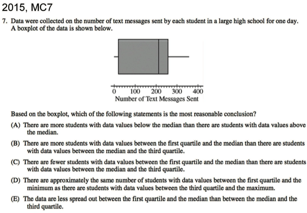
  选D

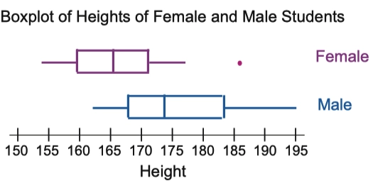
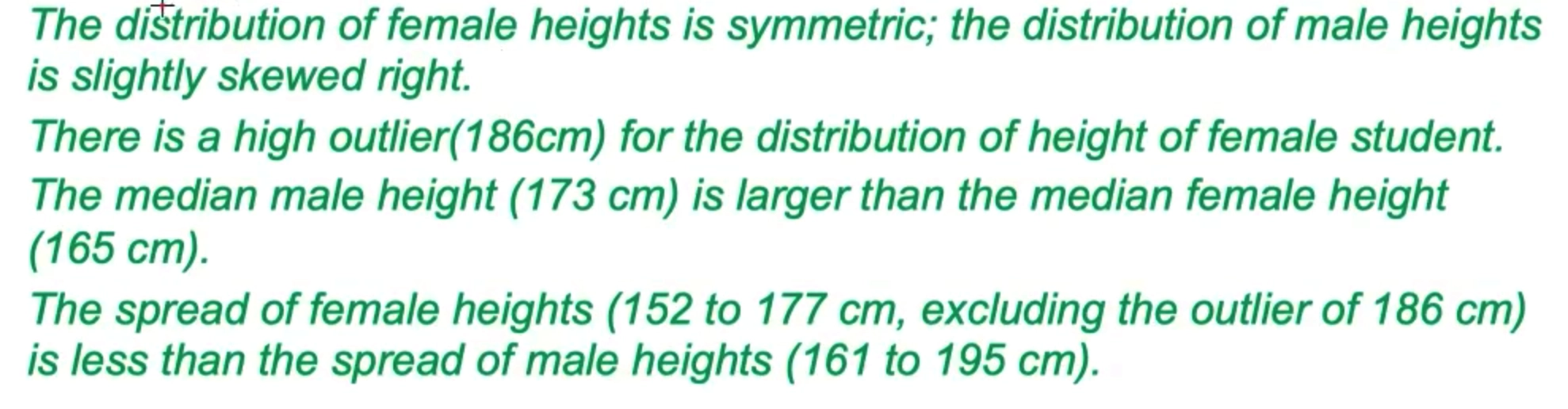
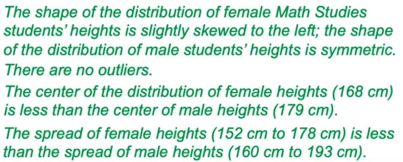
1.14.1 Comparison of Side-by-side Boxplot Graph 平行箱型图间的比较

• We should describe the side-by-side boxplot graph through four sides, SOCS.

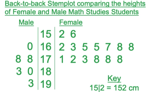
1.15.2 Comparison of Back-to-back Stemplot Graph 背对背茎叶图的比较

1.16 Effect of Transforming Data for Statistic Value 变换数据对统计数值的影响

1.16.1 Effect of Adding 数据加法变换的影响

• We add same number \(a\) to each observation of data set.
• This transformation of data would change the center and location (Mean, Median, Quartiles), and the changing size is \(a\). So, if the center and location is \(n\) before the transformation of data, then, the results of the transformation are \(n + a\)
• This transformation doesn’t affect the measures of spread (range, IQR, \(S_x\)) and doesn’t change the shape of the distribution.
• Adding transformation also doesn’t affect the Z-scores of data point.

\[z_i = \frac{x_i - \mu}{\sigma} \Rightarrow z_{\text{after}} = \frac {x_i + b - (\mu + b)}{\sigma} = z_i\]

1.16.2 Effect of Multiplying 数据乘法变换的影响

• We multiply same number \(b\) to each observation of data set.
• This transformation of data would change the center and location (Mean, Median, Quartiles) by \(\times b\), and also would change the measures of spread by \(\times |b|\)
• This transformation doesn’t affect the shape of the distribution, but it would make data more dispersion or concentration which depends on \(|b| > 1\) or \(0 > |b| > 1\)
• Multiplying transformation also doesn’t affect the Z-scores of data point.

\[z_i = \frac{x_i - \mu}{\sigma} \Rightarrow z_{\text{after}} = \frac {bx_i - b\cdot\mu}{b\cdot\sigma} = z_i\]

• In conclusion,

  • \(\mu_Y = b+a\mu_X\)
  • \(\sigma^2_Y = a^2\sigma^2_X\)
  • \(\sigma_Y = |a|\sigma_X\)

• Example

  

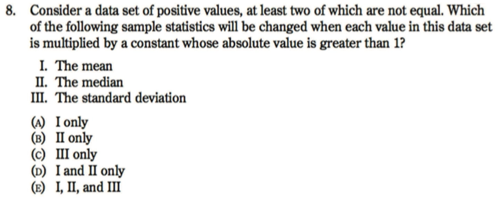
  选E

Unit 2: Exploring Two-Variable Data 双变量数据探索

2.1 Scatterplots and Correlation 散点图与关系

2.1.1 Basic Terms 基础术语

• Explanatory Variable and Response Variable
  • Assume we have a function \(h = \frac 12 gt^2\), where \(g\) is constant which is gravitational acceleration.
  • So we call \(t\) is the explanatory variable, and \(h\) is the response variable.
  • A response variable measures an outcome of a study.
  • An explanatory variable may help explain or influence changes in a response variable.

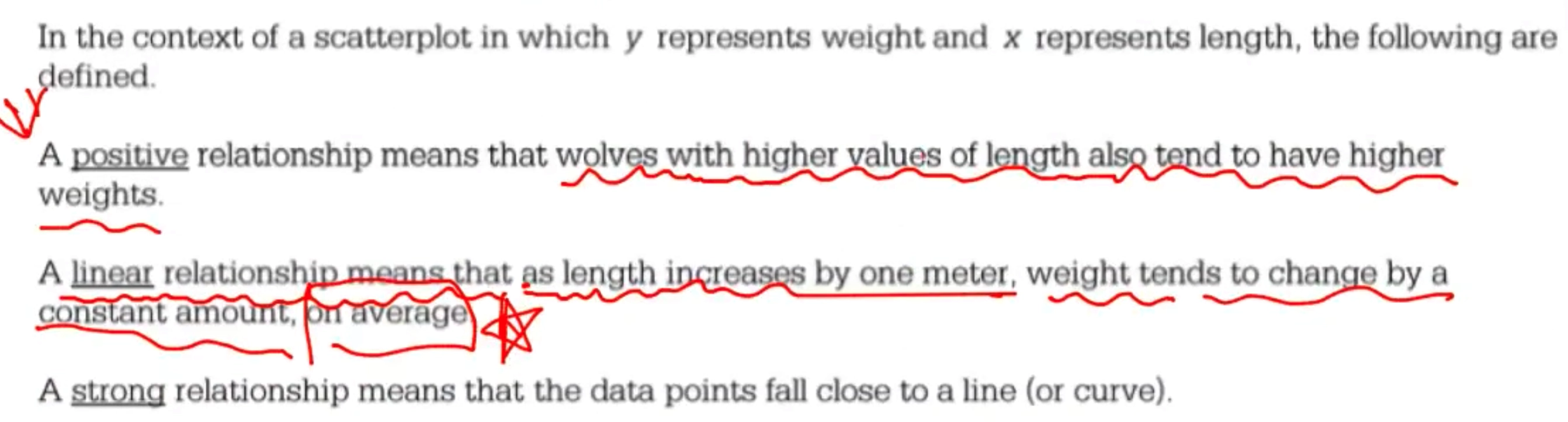
2.1.2 Displaying Relationships by Scatterplots 通过散点图来表示变量之间的关系

• A scatterplot shows the relationship between two quantitative variables measured on the same individuals. The values of one variable appear on the horizontal axis, and the values of the other variable appear on the vertical axis.
• Each individual in the data appears as a point on the graph.

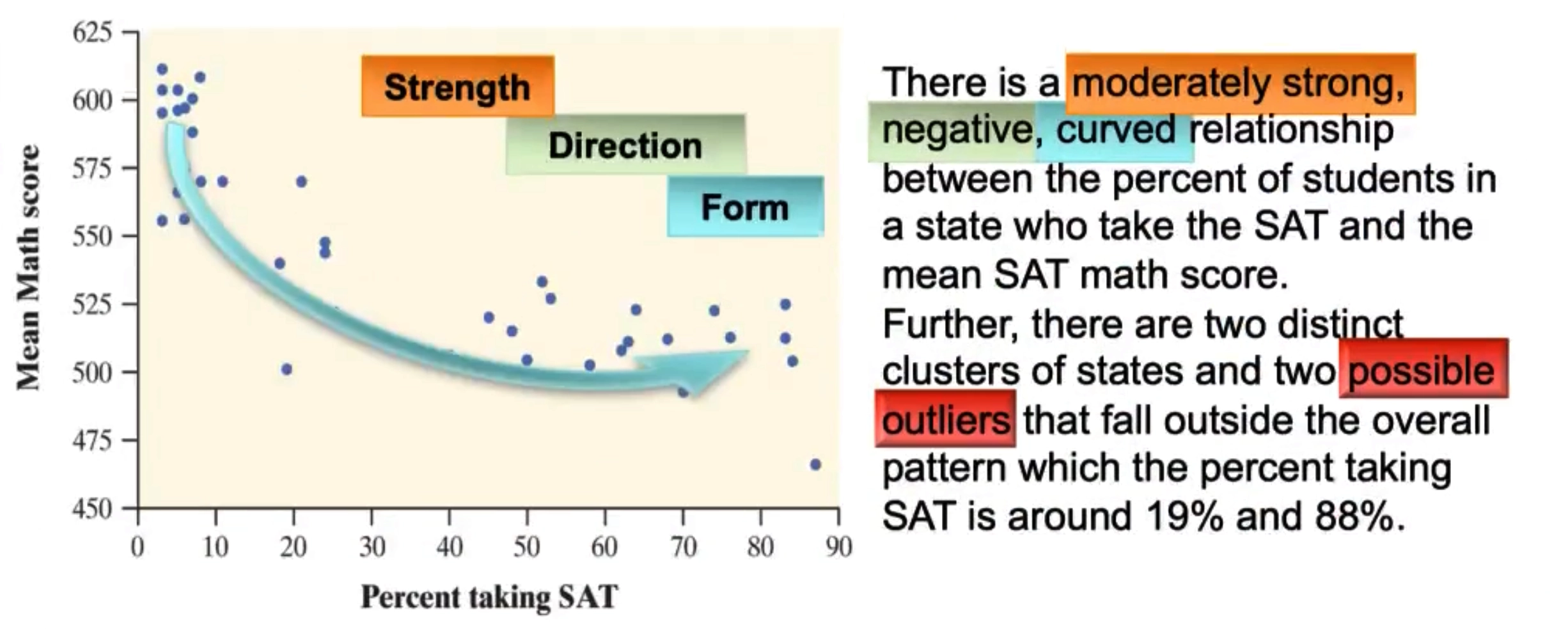
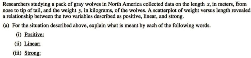
2.1.3 Interpreting Scatterplots 解释散点图

• We can describe the overall pattern of a scatterplot by the direction, form, and strength of the relationship.

• An important kind of departure is an outlier, an individual value that falls outside the overall pattern of the relationship.

• Direction: Positive or Negative

• Form: Linear or Nonlinear

• Strength (Fit of data points): Strong, Moderate, Weak

• Outliers: Location

• Example

  DFSO, four sides

  

  

  

  

  

2.1.4 Measuring Linear Association: Correlation

• A scatterplot displays the strength, direction, and form of the relationship between two quantitative variables.
• Linear relationships are important; meanwhile, our eyes are unfortunately not good judges of how strong a linear relationship is, so we should introduce another concept, called “Correlation \(r\)”.

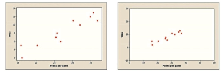
2.1.5 The Relationship between Correlation Coefficient and Linear Direction and Strength 相关系数与线性方向与强度的关系

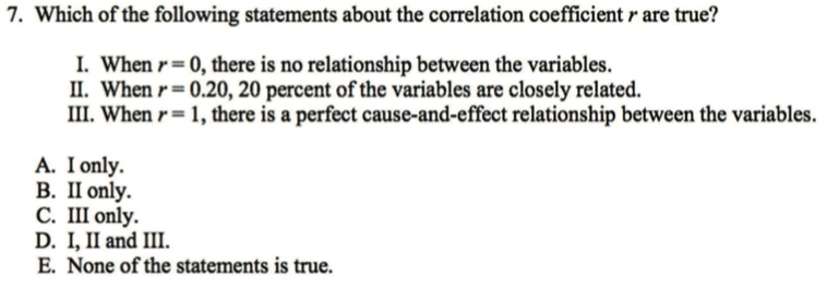
• The correlation \(r\) is a measure of the direction and strength of the linear relationship between two quantitative variables.

• Range: \(-1 \leq r \leq 1\)

• \(r > 0\) indicates a positive association, \(r < 0\) indicates a negative association.

• Values of \(r\) near \(0\) indicate a very weak linear relationship.

• The strength of the linear relationship increases as \(r\) moves away from \(0\) towards \(-1\) or \(1\).

• The extreme values \(r = -1\) and \(r = 1\) occur only in the case of a perfect linear relationship.

• Similarity, the interpretation of correlation \(r\) is as same as the interpretation of scatterplots.

• Example

  

2.1.6 How to Calculate the Correlation \(r\) 如何计算相关系数 \(r\)

• Calculate correlation \(r\) in sample

\[r =\frac 1{n-1}\cdot\sum^n_{i=0}(\frac{x_i - \bar x}{s_x})(\frac{y_i - \bar y}{s_y})\]

• Calculate correlation \(r\) in total population

\[r =\frac 1{n-1}\cdot\sum^n_{i=0}(\frac{x_i - \mu}{\sigma})(\frac{y_i - \mu}{\sigma}) = \frac 1{n-1}\cdot\sum^n_{i=0} z_x\cdot z_y\]

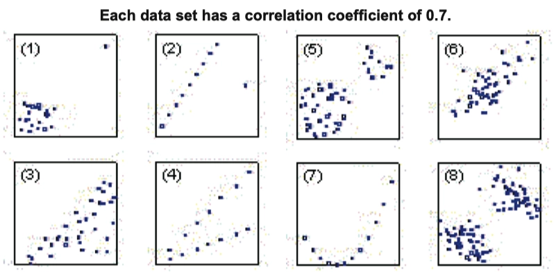
2.1.7 Facts about Correlation \(r\) 相关系数的性质

• Correlation makes no distinction between explanatory and response variables.

  • Correlation doesn’t imply causation.

• \(r\) does not change when we change units of measurement of \(x\), \(y\), or both.

  • Since adding and multiplying transformation would not affect Z-scores, it also could not affect correlation \(r\).

• The correlation \(r\) itself has no unit of measurement. It is just a number.

• Since correlation \(r\) includes mean and standard deviation, \(r\) is nonresistance.

• Example

  

  选 E

Before you use correlation \(r\) to judge the strength or direction of data set, you should determine the scatterplot is linear relationship.

• Practice: E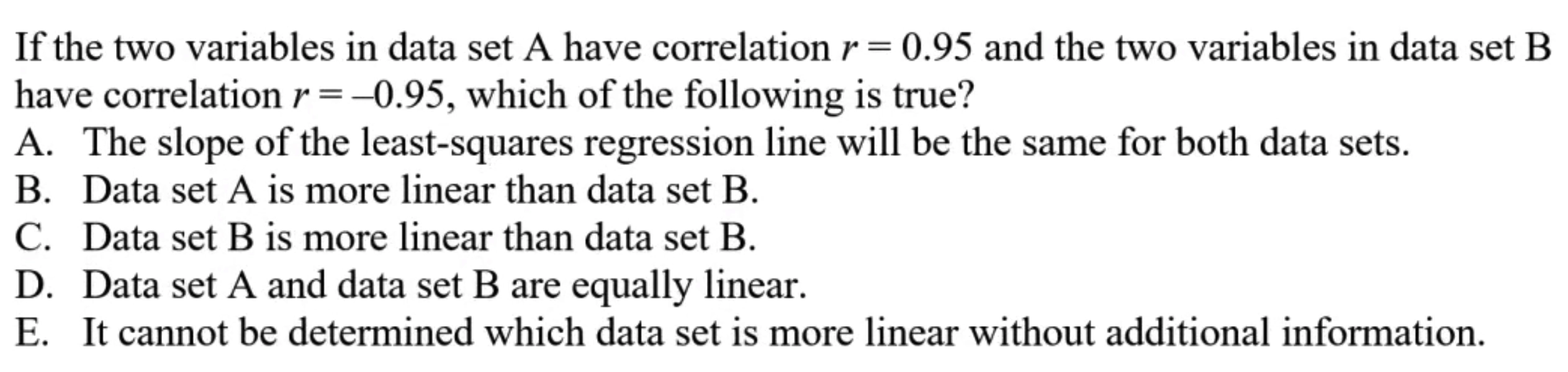

  

2.2 Least-Squares Regression 最小二乘回归

• A regression line summarizes the relationship between two variables, but only in settings where one of the variables helps explain or predict the other.

2.2.1 Residual and Residual Plots 残差与残差图

• A residual is the difference between an observed value of the response variable and the value predicted by the regression line.

\[\text{Residual} = y_{\text{observed}} - y_{\text{predicted}} = y - \hat y\]

• Residual could be positive or negative.
• A residual plot is a scatterplot of the residuals against the explanatory variable. Residual plots help us assess how well a regression line fits the data.
• And residual plot has following several facts if the residual plot could represent a strong linear relationship:
  • The residual plot should show no obvious patterns.
  • The residuals should be relatively consistent in size.
  • The residuals should be relatively small.

2.2.2 Least-Squares Regression Line 最小二乘回归线

• The least-squares regression line of \(y\) on \(x\) is the line that minimizes the sum of the squared residuals.

\[\min{\sum^n_{i=0}(y_i-\hat y_i)^2}\]

• We could calculate \(b\) and \(a\) in regression line equation \(\hat y = bx +a\).

\[b = r\cdot\frac{s_y}{s_x} \;,\; a = \bar y - b\bar x\]

• \((\bar x, \bar y)\) is always on the regression line \(\hat y\).

• Least-Squares Regression could imply causation.

• Since Least-Squares Regression includes \(r\) in computation progression, so regression line is also nonresistance.

• An outlier in regression is a point that does not follow the general trend shown in the rest of the data and has a large residual.

• A high-leverage point in regression has a substantially larger or smaller x-value than the other observations have.

• An influential point in regression is any point that, if removed, changes the relationship substantially. Examples include much different slope, y-intercept, and/or correlation. Outliers and high leverage points are often influential point.

• Example

  

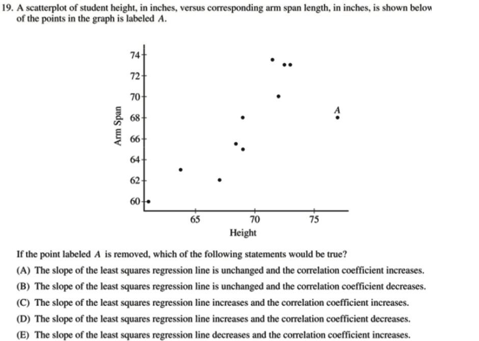
  选 C

2.2.3 Interpreting a Regression Line 解释一条回归线

• Regression Line Equation

\[\hat y = bx + a\]

• \(\hat y\) is the predicted value of the response variable \(y\) for a given value of the explanatory variable \(x\).
• \(a\) is the \(y\) intercept, the predicted value of \(y\) when \(x = 0\).
• \(b\) is the slope, the amount by which \(y\) is predicted to change when \(x\) increases by one unit, on average.

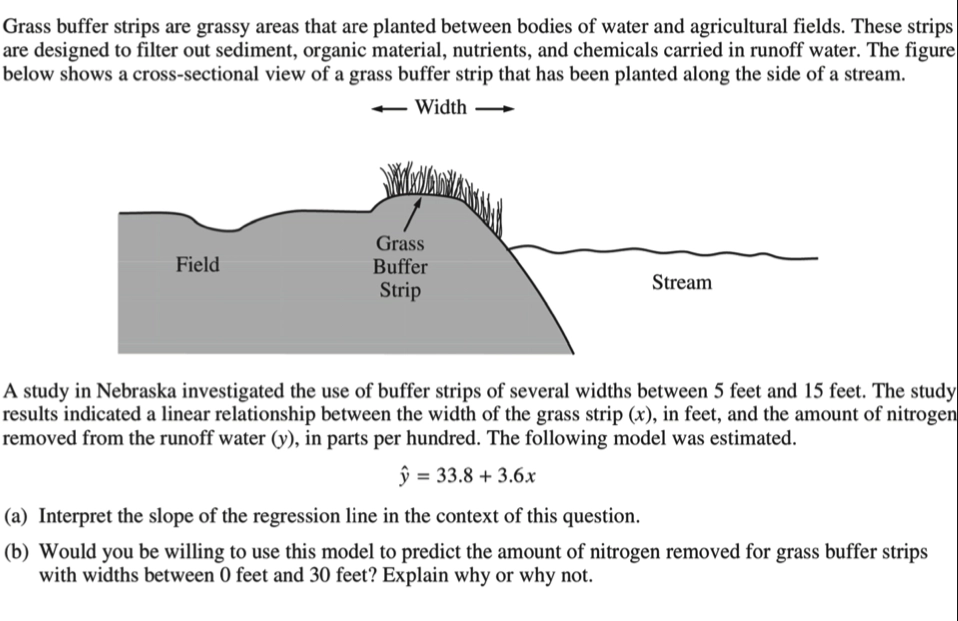
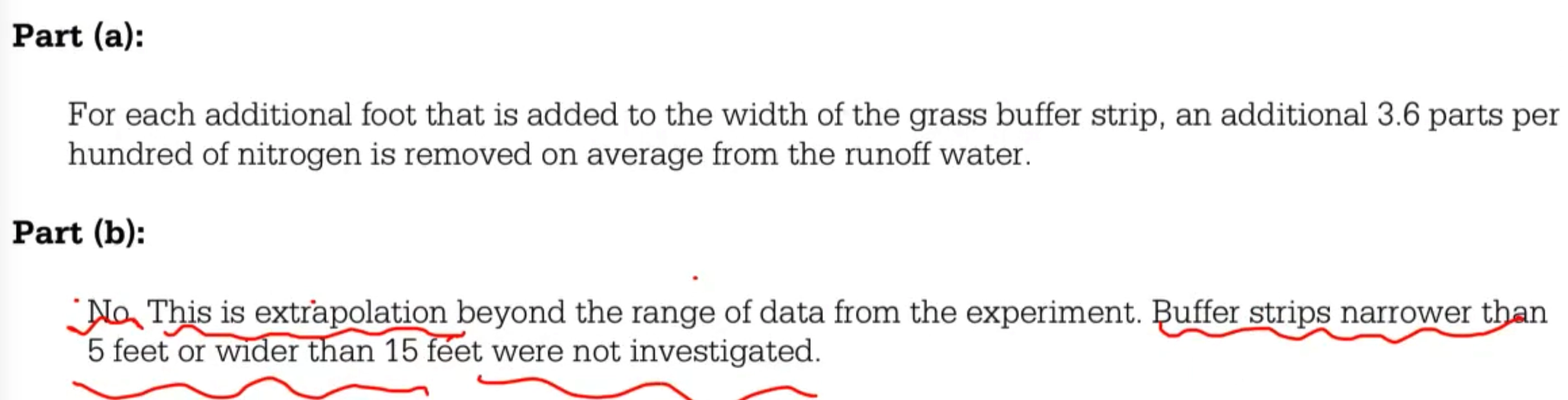
2.2.4 Extrapolation 外推

• Extrapolation is the use of regression line for prediction far outside the interval of values of the explanatory variable \(x\) used to obtain the line. Such predictions are often inaccurate.

• Example

  

  

2.2.5 The Role of \(s\) in Regression 残差标准差 \(s\) 在回归中的应用

• If we use a least-squares regression line to predict the values of a response variable \(y\) from an explanatory variable \(x\), the standard deviation of the residuals (\(s\)) is given by following

\[s = \sqrt{\frac1{n-2}\cdot\sum^n_{i=0}(y_i - \hat y)^2} = \sqrt{\frac{\sum^n_{i=0} \text{residuals}^2}{n-2}} = \sqrt{\frac {\text{SSE}}{n-2}}\]

2.2.6 The Role of \(r^2\) in Regression 判定系数 \(r^2\) 在回归中的应用

• The coefficient of determination \(r^2\), \(R^2\) (R-square) is the fraction of the variation in the values of \(y\) that is accounted for by the least-squares regression line of \(y\) on \(x\). We can calculate R2 using the following formula:

\[s^2 = R^2 = 1 - \frac{\text{SSE}}{\text{SST}} \\ \text{where, SSE} = \sum^n_{i=1}(y_i - \hat y)^2 = \sum^n_{i=0} \text{residuals}^2 \\ \text{and, SST} = \sum^n_{i=0} (y_i - \bar y)^2\]

• The SSE and SST in the formula, as shown above, are Sum of Squares due to Error and the Total Sum of Squares.

• Introduction of Another Error

  • MSE: Mean Squared Error

  \[\text{MSE} = \frac{\text{SSE}}{n} = \frac 1n\cdot\sum^n_{i=0}(y_i - \hat y_i)^2\]

  • RMSE: Root Mean Squared Error

  \[\text{RMSE} = \sqrt{\text{MSE}} = \sqrt {\text{SSE}/n} = \sqrt{\frac 1n\cdot\sum^n_{i=0}(y_i - \hat y_i)^2}\]

  • SSR: Sum of Squares of the Regression

  \[\text{SSR} = \sum^n_{i=0}(\hat y - \bar y)^2\]

Unit 3: Collecting Data 数据收集

3.1 Sample and Surveys 抽样与调查

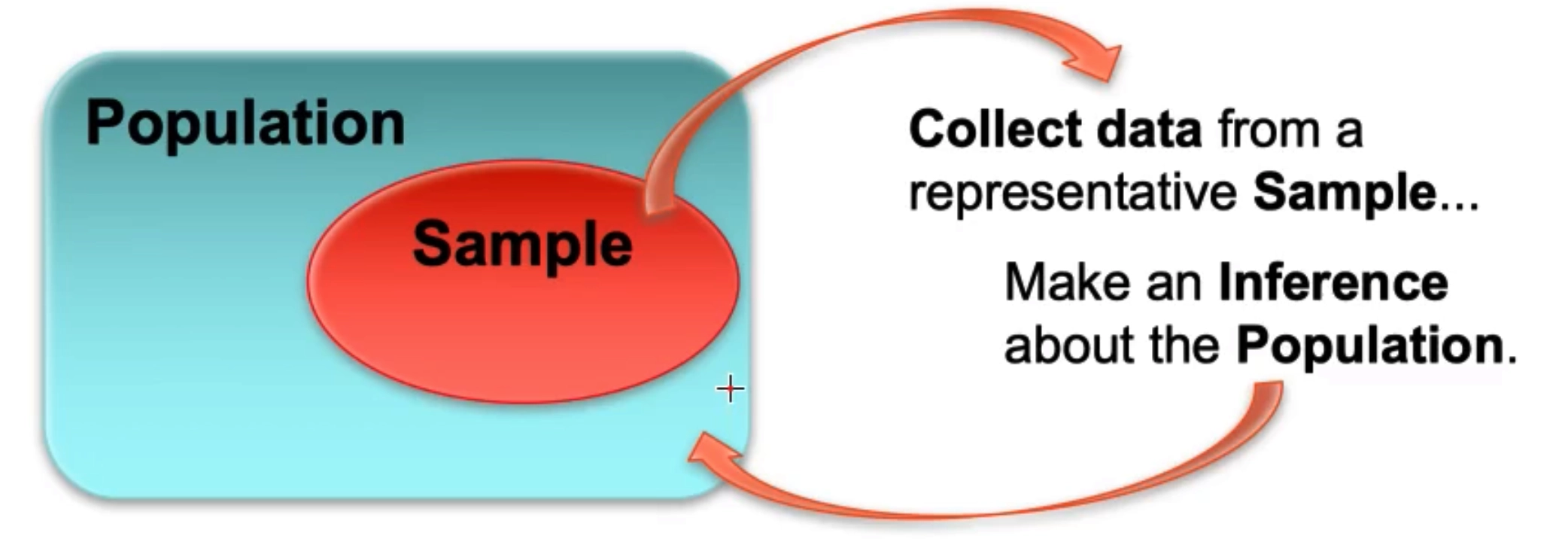
3.1.1 Population and Sample 总体与样本

• The population in a statistical study is the entire group of individuals we want information about.
• A sample is a subset of individuals in the population from which we actually collect data.

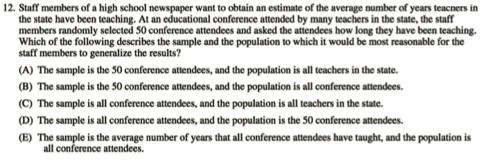
• Examples

  

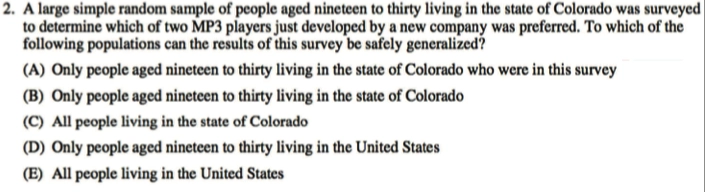
  选B

  

3.1.2 Census, and Sample Survey 普查与抽样调查

• A census collects data from every individual in the population.
  • Accurate, but expensive and sometimes is impossible.
• It is the intent of a sample survey to collect data from a representative portion of a population and to record the results.
  • Inaccurate, but saves time and labor.

3.1.3 Bad Sample Survey 不好的抽样调查方式

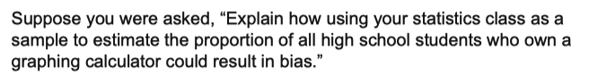
• Choosing individuals from the population who are easy to reach results in a convenience sample.

• The design of a statistical study shows bias if it would consistently underestimate or overestimate the value you want to know.

• A voluntary response sample consists of people who choose themselves by responding to a general invitation.

• Voluntary response samples show bias because people with strong opinions (often in the same direction) are most likely to respond.

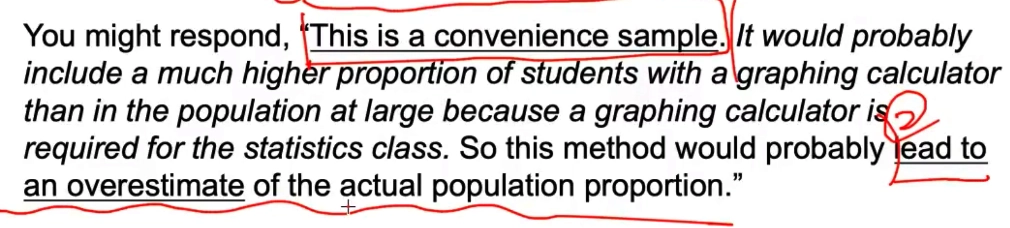
• Example

  

  

3.1.4 Correct Sample Survey 正确的抽样调查方式

• Random sampling involves using a chance process to determine which members of a population are included in the sample.

• Example

  

  选 A

3.1.5 Simple Random Sample (SRS) 简单随机抽样

• Step 1: Label, Give each member of the population a numerical label with the same number of digits.
• Step 2: Randomize. Use the table called Table D Random digits to randomly draw the samples.

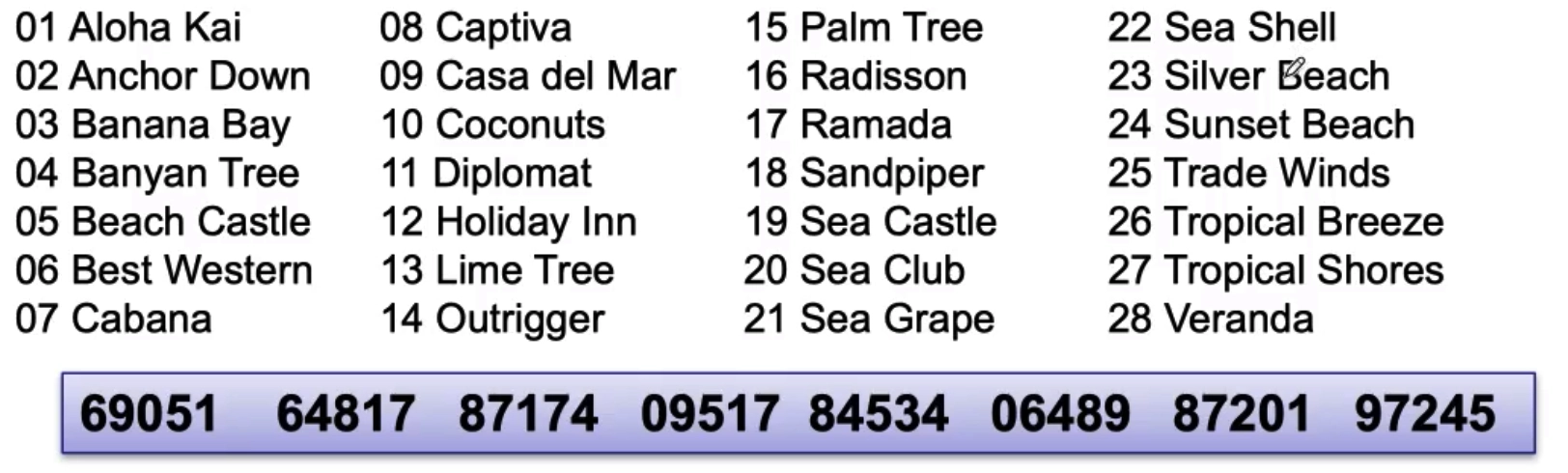
• As shown figure above, the maximum number of digits is 2 since the sample size is 28, so we take 2 digits per times to draw the samples. For example, 69 → does’t exist, 05 → Beach Castle, 16 → Radisson.
• 使得群内差异大，群间差异小

3.1.6 Stratified Random Sample 分层抽样

• To get a stratified random sample, start by classifying the population into groups of similar individuals, called strata.

• Stratified Random Sample can get less variability in the estimates since each characteristic of distinct strata can be evenly draw and to be representativeness.

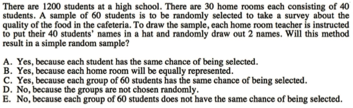
• Example

  

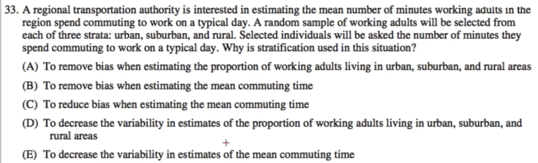
  答案为 E

3.1.7 Cluster Random Sample 种群抽样

3.1.8 Systematic Random Sample 系统抽样

• 间隔 \(n\) 个抽样

3.1.9 Bias on Survey 调查偏差

• Under coverage bias 覆盖不全偏差

• Nonresponse bias 不回答偏差

  • FRQ 中问到 Overestimate / Underestimate
    • 都可以说，但理由要合理，一般选 Overestimate 即回答了的人过拟合了

• Response bias 错误答案偏差

• Wording of question 问题偏差

• Example

  

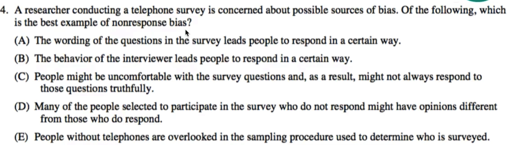
  答案为 D

3.2 Experiments 实验

• Experimental Study 有故意施加一些 treatment，然后去评估反应

  • 药物实验，分 Placebo 组和药物组，给药
  • 实验设计
    • 原则
      • 控制变量
      • 使用足够多可重复的 Experimental Units
    • 通过 Block 分组，抵消 Confounding 的影响（Block 内差异小）
    • Experimental Units → Treatment → Measure Response
    • Completely Randomized Design 完全随机设计
      • 分出对照组，随机抽人到不同的组别（类似 SRS）
    • Randomized Block Design 随机区组设计
      • 先按照类别分类，然后进行完全随机设计，随机抽分类后的人到不同的组别
    • Single-Blind 单盲实验
      • Placebo Effect 安慰剂效应
    • Double-Blind 双盲实验
      • 一些情况下双盲比较困难，操作无法隐藏，比如两种药的比较，打针和吃药（也可以同时打针和吃药隐藏操作）
    • Matched Pairs Design 配对设计
      • 最重要的是 Pairs 内相似
      • 2 treatment, 2 units
        • 夫妻，兄弟
      • 2 treatment, 1 unit
        • 先后顺序不同的两个操作
      • 1 treatment, 1 unit
        • 操作后对 unit 的前后比较
  • 可以说明因果关系 Casual Relationship

  

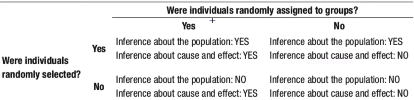
  推知总体 / 因果关系 与 样本是否随机选取，实验是否随机分组 有关

• Observational Study 是只观测存在的数据

  • 调查吸烟与肺癌的关系，取吸烟组与不吸烟组进行对照比较
  • 只能表面有关联 Association，但是不能说明因果 Casual Relationship

Unit 4: Probability 概率

4.1 Randomness, Probability, and Simulation 随机，概率和模拟

• 大数定理 Law of Large Number: 模拟次数足够多，就可以趋近真实概率值

If we observe more and more repetitions of any chance process, the proportion of times that a specific outcome occurs approaches a single value.

4.2 Probability Rules 概率规则

• Sample Space 样本空间 \(S\)，所有可能结果的集合

Set of all possible outcomes.

• Probability Model 概率模型 \(P(X)\)，对于样本空间的每一个元素 \(X\)，可以给定概率为 \(P(X)\)
• Legitimate Values 对于同一概率模型下的概率应符合以下规则

\[ 0 \leqslant P(A) \leqslant 1 \]

\[ \sum\limits_{i} P_i = 1 \]

\[ P(A^{C}) = 1 - P(A) \]

• Event 事件， 满足一些特定条件 所有可能结果的集合
  • 例如投骰子，样本空间 \(S = \{1,2,3,4,5,6\}\) 那么对于每一个 \(S\) 中的元素存在 \(P(X) = \frac 16\)
  • 投出大于 \(3\) 的数字所有可能的集合便是 \(S = \{4, 5, 6\}\)，那么 \(P(X > 3) = \frac 36 = \frac 12\)

4.3 Conditional Probability and Independence 条件概率和事件独立性

• 对于互斥事件
  • \(P(A \cup B) = P(A) + P(B)\)
  • \(P(A \cap B) = 0\)
• 对于非互斥事件
  • 对于独立事件
    • \(P(A\cap B) = P(A) + P(B) - P(A \cup B) = P(A)P(B)\)
    • \(P(A|B) = P(A)\)
  • 对于非独立事件
    • \(P(A\cap B) = P(A) + P(B) - P(A \cup B) = P(A)P(B|A)\)
    • \(P(A|B) = \frac{P(A \cap B)}{P(B)}\)

Unit 5: Discrete Random Variables and Probability Distributions 离散随机变量和概率分布

5.1 Binomial Distribution 二项分布

• 反复多次实验 \(n\) 次
• 实验与实验之间独立 Independent
• 实验结果分两类
  • Success
  • Failure
• 每次实验成功概率相同
• \(X\) 代表的是，在 \(n\) 次实验中，成功的概率为 \(P\)
• \(P(X=k)=\begin{pmatrix}n \\ k\end{pmatrix} p^k(1-p)^{n-k}\)
• \(\mu_x = np\)
• \(\sigma_x = \sqrt{np(1-p)}\)

5.2 Geometric Distribution 几何分布

• 反复多次实验 \(n\) 次
• 实验与实验之间独立
• 实验结果分两类
  • Success
  • Failure
• 每次实验成功概率相同
• \(Y\) 代表的是，总共 \(n\) 次实验，前面第 \(Y-1\) 都失败，第 \(Y\) 次成功的概率为 \(P\)
• \(P(X = k) = (1-p)^{k-1}p\)
• \(\mu_y = \frac 1p\)
• \(\sigma_y = \frac {\sqrt{1-p}}{p}\)

Unit 6: Continuous Random Variables and Probability Distributions 连续随机变量和概率分布

6.1 Normal Distribution 正态分布

• 单峰，对称，钟形
• 经验法则（Empirical Rule）\(68\%, 95\%, 99.7\%\)
• 通过 \(\text{Z-score}\) 对正态分布进行标准化处理 \(z=\frac{x - \mu}{\sigma}\)
  • 任何正态分布上的 \(x\) 都可以通过标准化转换到标准正态分布 即 \(X \sim N(0,1)\)
• Sample Distribution: \(\bar x \sim N(\mu, \frac{\sigma}{\sqrt n})\)

6.2 Linear Transformation of Normal Distribution 正态分布的线性变换

• 区分正态分布的线性变换和组合
  • Linear Transformation 线性变换
    • \(a\cdot\sigma_T = \sqrt{a^2 \cdot \sigma_X^2}\)
  • Combination 组合
    • \(\sigma_T = \sqrt{\sigma_X^2 + \sigma_Y^2}\)

Unit 7: Sampling Distribution 样本分布

• Parameter，用于描述总体的特征（统计量），通常不清楚
• Statistic（Estimator，Point Estimator），用于描述样本的特征（统计量），通常用 Statistic 推断 Parameter
• 如果是 Categorical Variable 通常使用样本的比例（Proportion）估进行计计
  • Parameter Proportion: \(p\)
  • Statistic Proportion: \(\hat p\)
• 如果是 Quantitative Variable 则通常使用样本的均值进行估计
  • Parameter Mean: \(\mu\)
  • Statistic Mean: \(\bar x\)
• 中心极限定理 \(n \to \infty\), \(\sigma \to 0\)
• 通过增大样本量减少 variability of statistic
• 必须是随机的 unbiased 调查 estimator mean 才能等于 parameter

Condition of Sampling Distribution 抽样分布的条件

• Sampling Proportion Distribution: \(\hat p \sim N (p, \sqrt{\frac{p(1-p)}{n}})\)
  • Random Condition: 从题目摘抄, “The sample is randomly selected. (…)”
  • Large Count Condition of Proportion: \(\begin{cases} np \geq 10 \\ n(1-p) \geq 10 \end{cases}\)
  • Two Sample: \(\mu_{X-Y} = p_X - p_Y\), \(\sigma_{X-Y} = \sqrt{\frac{p_1(1-p_1)}{n_1} + \frac{p_2(1-p_2)}{n_2}}\)
• Sampling Mean Distribution: \(\bar x \sim N(\mu, \frac{\sigma}{\sqrt n})\)
  • Large Count Condition of Mean:
    • \((n < 30)\) We can assume the population is normally distribution.（或者一定要找到题目中关于 Sampling Distribution 是正态分布的假设或证据
    • \((n \geq 30)\) Because the sample is large, based on CLT, the sampling distribution of sample mean is approximately normal.
  • Matched-Pair Two Sample: \(\mu_{X-Y} = \mu_X - \mu_Y\), \(\sigma_{X-Y} = \sqrt{\frac{\sigma^2_X}n + \frac{\sigma_Y^2}n}\)
• Independent - \(n \leq \frac 1{10} N\) （没有提供 \(N\) 就需要其他角度表述题目的背景符合 Independent）

Unit 8: Estimating with Confidence 置信估计

• 置信区间 Confidence Interval: \(\text{estimate} \pm \text{margin of error} = \text{estimate} \pm \text{crtical value} \times \text{std of statistic}\)
  • \(\text{estimator} = \frac{\text{upper bound} + \text{lower bound}}{2}\)
  • \(\text{margin error} = \frac{\text{lower bound} - \text{upper bound}}{2}\)
• 通过在 Population 中，以 \(\mu\) 为中心，设置 Confidence Level 置信水平
  • 置信水平代表的是 Sample 落在置信区间里的可能
  • 然后以 Sample 的 \(\bar x\) 为中心，构造置信区间，只要 Sample 落在置信区间，就必可以 Capture 到总体 \(\mu\)
  • 增加置信水平，置信区间就会增加，相应的减少置信水平，置信区间就会减少，所以无论如何，精确度取决于样本量 \(n\)
• 最小样本量问题 \(z^*\cdot (\frac{\sigma}{\sqrt n}) \leq ME\), \(z^*\cdot \sqrt{\frac{\hat p (1-\hat p)}{n}} \leq ME\) （没给 \(p\) 默认 \(0.5\)）
• 总体均值问题
  • 总体分布是正态分布
    • \(n < 30\), \(\sigma\) is known
      • Mean
      • Proportion
    • \(n < 30\), \(\sigma\) is unknown
  • 总体分布不知道或者是偏分布
• 使用 Confidence Intervals 同样需要严格遵守 Sampling Distribution Condition
• FRQ Template
  • State: Method + In context
    • \(\text{one/two}\) sample \(z/t\) interval for \(\mu \; / \; \mu_X - \mu_Y\)
    • where \(\mu \; / \; \mu_X - \mu_Y\) denotes the \(\text{[In context]}\)
  • Plan: Condition
  • Do: Calculate Confidence Interval
  • Conclude: Interpret Confidence Interval
    • Confidence Level Interpret
      • The \(C\%\) confidence level means that if one were to repeatedly take random samples of the same size from the population and construct a \(C\%\) confidence interval from each sample, then in the long run \(C\%\) of those intervals would succeed in capturing the actual value of the \(\text{[population parameter in context]}\).
    • Confidence Interval Interpret
      • We are \(C\%\) confident that the interval from \(\text{upper bound}\) to \(\text{lower bound}\) captures the actual value of the \(\text{[population parameter in context]}\).
• Matched-Pairs: \(t\) distribution, 使用 \(\mu_d\)

Unit 9: Testing a Claim

• 原假设 / 零假设 null hypothesis，\(H_0\)
• 备选假设 alternative hypothesis，\(H_a\)

• \(\text{test statistic} = \frac{\text{statistic }-\text{ parameter}}{\text{standard deviation of statistic}}\)
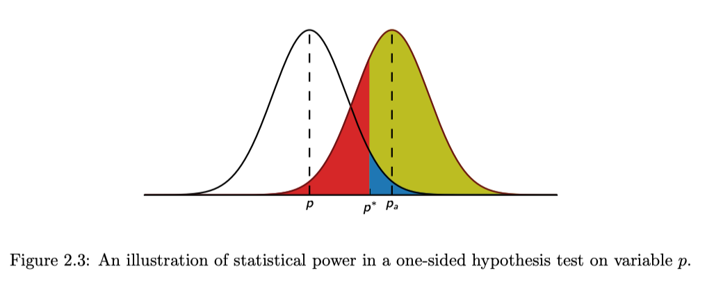
• 可以认为，我们基于 \(H_0\) 正确的情况下，观测值应该的分布（图中左边的分布），所以我们通过 \(\text{test statistic}\)，将我们实际得到的观测值变换到左边的分布下。（就相当于是做极端程度的标准化）
  • 所以，如果我们实际得到的观测值，在观测值应该的分布上与中心偏差极大，大到超过「显著性水平」（图中的 \(p^*\)，那便说明我们实际得到的观测值，可能不符合，在假设 \(H_0\) 为正确的情况下的分布，所以我们拒绝 \(H_0\)。
  • 注意，我们不能说接受 \(H_0\) 或者 \(H_a\)，因为在推断统计的框架下一切只能是概率的情况下，只能说「不能拒绝 Fail to reject it」或者「拒绝 Reject it」假设
• Type I Error \(\alpha\): 实际在 \(H_0\) 分布下，但 \(p < p^*\)，图中蓝色部分，也就是 \(H_0\) 是对的但是被拒了的概率（拒真错误）
• Type II Error \(\beta\): 实际在 \(H_a\) 分布下，但 \(p > p^*\)，图中红色部分，也就是 \(H_0\) 是错的但是没被拒的概率（受伪错误）
  • Power: \(1 - \beta\): 没有 Type I, II Error 的情况下在且实际上 \(H_a\) 是对的概率，图中黄色 + 蓝色的部分，同样是概率
• 显著性水平 Significance Level \(\alpha\)
  • \(H_0:\text{parameter} = \text{claimed value}\)
  • Right-tailed Test
    • \(H_a: \text{parameter} > \text{claimed value}\)
    • \(Z > Z_\alpha\), reject \(H_0\)
  • Left-tailed Test
    • \(H_a: \text{parameter} > \text{claimed value}\)
    • \(Z < -Z_\alpha\), reject \(H_0\)
  • Two-tailed Test
    • \(H_a: \text{parameter} \neq \text{claimed value}\)
    • \(Z > Z_\alpha \text{ or } Z < -Z_\alpha\), reject \(H_0\)
      • \(|Z| > Z_\alpha\), reject \(H_0\)
  • \(\text{p-value} < \alpha\), reject \(H_0\)
    • \(\text{p-value}\) 是在假设 \(H_0\) 为真的情况下，比观测值还极端的概率
• Type I Error: \(H_0\) 为真，但 \(H_0\) 被 reject
• Type II Error: \(H_0\) 为假，但 \(H_0\) fail to reject
• Type I, II Error 此消彼长
• Power: \(1 - \beta\)
  • Increase \(n\)
  • Increase \(\alpha\)
• Condition 和 CI 一样
• FRQ
  • State: \(H_0\) and \(H_a\), parameter in context
  • Plan: RNI
  • Do: Calculate p-value
  • Conclude: Interpret p-value
    • p-value Interpret
      • Because the p-value of \([p]\) is larger than any reasonable significance level, such as \(\alpha = .05\), do not reject the null hypothesis that the mean number of \(\text{[mean in context]}\). There is not sufficient evidence to conclude that the \([H_a]\)

Unit 10: Inference for Categorical Data Chi-Square

• 单变量 One-variable
  • 拟合优度假设检验 Chi-Square Goodness-of-fit Test
    • \(\text{test statistic} = \sum\frac{(\text{observed} - \text{expected})^2}{\text{expected}}\)
    • 非负值
    • Condition: RLI
      • Large Sample Size: All expected counts are at least 5
• 双变量 Two-variable
  • \(df = (\text{row} - 1)(\text{col} - 1)\)
  • \(\text{expected count} = \frac{\text{row} \times \text{col}}{\text{total}}\)
  • Chi-Square Test for Homogeneity
    • 用于实验
    • \(H_0\): no difference
    • \(H_a\): difference
  • Chi-Square Test for Association / Independence
    • 用于调查
    • \(H_0\): independent
    • \(H_a\): not independent

Unit 11: Inference for Quantitative Data Slopes

• \(b \sim N(\beta, \frac{\sigma_y}{\sigma_x\sqrt n})\), \(SE_b = \frac{s_y}{s_x\sqrt{n-1}}\)

Sample Inference Summary

• Population Mean
  • Population Distribution is Normal
    • (小样本) \(n < 30\), \(\sigma\) is known (z-interval)
      • Mean
      • Proportion
    • (小样本) \(n < 30\), \(\sigma\) is unknown (t-interval)
      • Mean
      • Proportion
  • Population Distribution is Skewed or Unknown
    • (大样本) \(n \geq 30\), CLT, \(\sigma\) is unknown
      • Mean
      • Proportion
    • (小样本) \(n < 30\), CLT, \(\sigma\) is unknown
      • Mean
      • Proportion
• Population Difference Mean
• Sampling Distribution of Sample
  • Population Distribution is Normal
    • Mean
      • \(\bar x \sim N(\mu, \frac{\sigma}{\sqrt n})\)
    • Proportion
  • Population Distribution is Skewed / Unknown
    • Mean
      • \(n \geq 30\), CLT
    • Proportion
• Sampling Distribution of Difference of Sample Mean
  • Both population distribution is normal
  • Both population distribution is skewed / unknown
    • Mean
      • \(n_1 \geq 30,\, n_2 \geq 30\), CLT
• Sample Proportion
• Difference Proportion

FRQ Quick Sheet

Linear Transformation

• Add \(n\)
  • \(\mu, Q_n + a\)
• Multiple \(b\)
  • \(\mu, Q_n \times b\)
  • \(\sigma_Y = |b|\sigma_X\)

Regression

• Strong Relation → Residual
  • Show no obvious patterns
  • Relatively consistent in size
  • Relatively small
• Correlation doesn’t imply causation
• Sum of Residuals = 0
• 调换 \(x,y\) 不影响 \(r\)
• \(r\) 不受到线性变换的影响
• 用 \(r\) 之前先确定线性关系
• \((\bar x, \bar y)\) 一直都在 \(\hat y\) 上
• Outlier → Residual Large
• High-leverage → X Large
• Influential Point → Huge Effect on Slope
• 只能预测数据范围内的不能外推 Extrapolation

FRQ Template

• Describe the Distribution
  • SCOS Shape Outlier Center Spread
  • Shape: The distribution of \(\text{[in context]}\) is normal / skewed to left / right.
  • Outlier: There is a gap between the \(\text{[in context]}\).
  • Center: The median \(\text{[in context]}\) is ….
  • Spread: The data vary from a minimum of … to a maximum of …
• Compare the Distribution
  • Variability, Shape
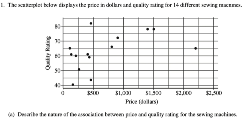
• Scatter Point
  • Direction: Positive or Negative
  • Form: Linear or Nonlinear
  • Strength (Fit of data points): Strong, Moderate, Weak
  • Outliers: Location
• Regression Line Equation
  • \(\hat y\) is the predicted value of the response variable \(y\) for a given value of the explanatory variable \(x\).
  • \(a\) is the \(y\) intercept, the predicted value of \(y\) when \(x = 0\).
  • \(b\) is the slope, the amount by which \(y\) is predicted to change when \(x\) increases by one unit, on average.
  • \(r^2\) 有多少 \(y\) 的 Variability 可以被 x 解释
• FRQ
  • State: \(H_0\) and \(H_a\), parameter in context
  • Plan: RNI
  • Do: Calculate p-value
  • Conclude: Interpret p-value
    • p-value Interpret
      • Because the p-value of \([p]\) is larger than any reasonable significance level, such as \(\alpha = .05\), do not reject the null hypothesis that the mean number of \(\text{[mean in context]}\). There is not sufficient evidence to conclude that the \([H_a]\)
• FRQ
  • State: Method + In context
    • \(\text{one/two}\) sample \(z/t\) interval for \(\mu \; / \; \mu_X - \mu_Y\)
    • where \(\mu \; / \; \mu_X - \mu_Y\) denotes the \(\text{[In context]}\)
  • Plan: Condition
  • Do: Calculate Confidence Interval
  • Conclude: Interpret Confidence Interval
    • Confidence Level Interpret
      • The \(C\%\) confidence level means that if one were to repeatedly take random samples of the same size from the population and construct a \(C\%\) confidence interval from each sample, then in the long run \(C\%\) of those intervals would succeed in capturing the actual value of the \(\text{[population parameter in context]}\).
    • Confidence Interval Interpret
      • We are \(C\%\) confident that the interval from \(\text{upper bound}\) to \(\text{lower bound}\) captures the actual value of the \(\text{[population parameter in context]}\).