11.1 Parametric Equations 参数方程

参数方程便是，\(x(t)\)，\(y(t)\)，都是关于另一个变量 \(t\) 的函数，例如

\[\begin{cases} x(t) = \cos(t) \\ y(t) = \sin(t) \end{cases} \quad 0\leq t\leq 2\pi\]

Eliminate the Parameter of Parametric Equation 参数方程的消参

• 例题

\(\text{(a)}\) 我们通过三角恒等式 \(\sin^2(\theta) + \cos^2(\theta) = 1\) 可以得到 \(x^2 + y^2 = 1\)

\(\text{(b)}\)

\[\begin{cases} x = 1-t \\ y = \sqrt t \end{cases} \; t \geq 0\]

我们可以通过两边同时开方，消掉 \(t\)

\[\begin{aligned} y^2 &= t \\ x &= 1-t = 1-y^2 \\ y^2 &= 1-x \end{aligned}\]

\(\text{(c)}\)

\[ \begin{cases} x = a \sin(t) \\ y = b \cos(t) \end{cases} \]

我们同样的想要得到类似 \(\sin^{2} (x) + \cos^{2} (x) = 1\) 的形式（容易去想 \(x^{2} + y^{2}\) 从而导致），所以我们将其整体平方

\[ \begin{cases} x^{2} = a^{2} \sin^{2} (t) \\ y^{2} = b^{2} \cos^{2} (t) \end{cases} \implies \begin{cases} \frac{x^{2}}{a^{2}} = \sin^{2} (t) \\ \frac{y^{2}}{b^{2}} = \cos^{2} (t) \end{cases} \]

最终得到

\[ \frac{x^{2}}{a^{2}} + \frac{y^{2}}{b^{2}} = 1 \]

\(\text{(d)}\)

\[ \begin{cases} x = 4e^{t} \\ y = 2e^{-t} \end{cases} \implies t=\ln \left(\frac{x}{4}\right) \implies y=2e^{-\ln \left(\frac{x}{4}\right)}=2\cdot \frac{4}{x} = \frac{8}{x} \]

Derivatives of Parametric Equation 参数方程的求导

如果可以消去参数，就是隐函数求导，例如上述 \(\text{(b)}\)

\[ y^2 = 1 - x \Rightarrow 2y\cdot y' = -1 \Rightarrow y' = -\frac{1}{2y} \]

如果不可以，则按照导数的定义式推导，譬如我们有以下参数方程

\[ \begin{cases} x = x(t) \\ y = y(t) \end{cases} \]

我们可以得到

\[ \frac{\mathrm{d}y}{\mathrm{d}x} = \frac{\frac{\mathrm{d}y}{\mathrm{d}t}}{\frac{\mathrm{d}x}{\mathrm{d}t}} = \frac{y'(t)}{x'(t)} \]

• 例题

\(\text{(a)}\) 求 \(t = \frac{\pi}{2}\) 处斜率

\[ \begin{cases} x = a (t - \sin t) \\ y = a (1 - \cos t) \end{cases} \]

\[ \frac{\mathrm{d}y}{\mathrm{d}x} = \frac{\frac{\mathrm{d}y}{\mathrm{d}t}}{\frac{\mathrm{d}x}{\mathrm{d}t}} = \frac{a \sin t}{a - a \cos t} = \frac{\sin t}{1 - \cos t} \\ ~ \\ \therefore \frac{\mathrm{d}y}{\mathrm{d}x}\bigg|_{t=\frac{\pi}{2}} = \frac{\sin \frac{\pi}{2}}{1 - \cos \frac{\pi}{2}} = 1 \]

\(\text{(b)}\) 写出下列方程过点 \((1, \sqrt{2})\) 的切线方程

\[ \begin{cases} x = \tan(\theta) \\ y = \sec(\theta) \end{cases} \]

\[ \frac{\mathrm{d}y}{\mathrm{d}x} = \frac{y'(\theta)}{x'(\theta)} = \frac{\tan (\theta)}{\sec (\theta)} = \sin (\theta) \]

当 \(x = 1\) 时 \(\theta = \frac{1}{4} \pi\)，所以切线为

\[ y = \sin\left( \frac{1}{4} \pi \right) \cdot (x-1) + \sqrt{2} = \frac{\sqrt{2}}{2}\cdot (x - 1) + \sqrt{2} \]

Second Derivatives of Parametric Equation 参数方程的二阶导数

根据一阶导数可以推导得到

\[ \frac{\mathrm{d}^2y}{\mathrm{d}x^2} = \frac{\mathrm{d}}{\mathrm{d}x}\left( y' \right) = \frac{\frac{\mathrm{d}y'}{\mathrm{d}t}}{\frac{\mathrm{d}x}{\mathrm{d}t}} = \frac{\frac{\mathrm{d}\frac{\frac{\mathrm{d}y}{\mathrm{d}t}}{\frac{\mathrm{d}x}{\mathrm{d}t}}}{\mathrm{d}t}}{\frac{\mathrm{d}x}{\mathrm{d}t}} = \frac{\frac{\mathrm{d}\frac{y'(t)}{x'(t)}}{\mathrm{d}t}}{x'(t)} \]

• 例题

\(\text{(a)}\) \[ \begin{cases} x = 3t + 9 \\ y = \sin ^{2}(4t) \end{cases} \]

计算 \(\frac{\mathrm{d}y}{\mathrm{d}x}\)，以 \(t\) 表示

Hint: \(\sin (nt) + \cos (nt) = \sin (2nt)\)

\[ \frac{\mathrm{d}y}{\mathrm{d}x} = \frac{y'(t)}{x'(t)} = \frac{2 \sin (4t) \cos (4t) \cdot 4}{3} \]

\(\text{(b)}\)

\[ \begin{cases} x = \cos(2t) \\ y = -9 \cos(t) \end{cases} , \; 0 < t < \pi \]

计算 \(\frac{\mathrm{d}y}{\mathrm{d}x}\) 和 \(\frac{\mathrm{d}^{2}y}{\mathrm{d}x^{2}}\)，以 \(t\) 表示

Hint: \(\sin(2x) = 2 \sin(x) \cos(x)\)

\[ \frac{\mathrm{d}y}{\mathrm{d}x} = \frac{y'(t)}{x'(t)} = \frac{9 \sin(t)}{-2 \sin(2t)} = \frac{9 \sin(t)}{-2 \cdot 2 \cdot \sin (t)\cos (t)} = -\frac{9}{4 \cos(t)} \]

\[ \frac{\mathrm{d}^{2}y}{\mathrm{d}x^{2}} = \frac{\frac{\mathrm{d}\left( -\frac{9}{4 \cos(t)} \right)}{\mathrm{d}t}}{-2 \sin(2t)} = \frac{9 \sin (t)}{4 \cos^{2} (t)} \cdot \frac{9}{2 \cdot 2 \cdot \sin(t) \cos(t)} = \frac{9}{16 \cos^{3}(t)} \]

Area Under a Parametric Curve 参数曲线所围成的面积

对于 \(y = f(x)\) 我们可以轻松的得出他的曲线下面积公式

\[ A = \int_{a}^{b} f(x) ~\mathrm{d}x \]

但是对于参数方程 \(y(t), x(t)\)，我们可以进行如下等价变换

\[ f(x) \to y(t) \\ \mathrm{d}x \to x'(t) \\[0.8em] f(x)\cdot \mathrm{d}x \to y(t) \cdot x'(t) \]

所以我们可以得到

\[ A = \int_{a}^{b} y(t)x'(t) ~\mathrm{d}t \]

• 例题

\(\text{(a)}\) 求下列参数曲线所围的面积 \[ \begin{cases} x = 2 \cos(\theta) \\ y = 4 \sin(\theta) \end{cases} \quad 0\leqslant \theta \leqslant 2 \pi \]

Hint: \(\sin^{2}(x) = \frac{1}{2}(1 - \cos(2x))\)

\[ \int_{0}^{2\pi} 4 \sin(\theta) \cdot -2\sin(\theta) ~\mathrm{d}\theta = -8 \pi \]

因为面积是正的所以答案为 \(8 \pi\)

11.2 Arc Length of Parametric Equation 参数方程的弧长

若我们有以下参数方程

\[\begin{cases} x = x(t) \\ y = y(t) \end{cases}\]

其中 \(x(t)\)，\(y(t)\) 在 \([a, b]\) 区间中连续且可导

\[ \begin{aligned} \mathrm{d}s &= \sqrt{(\mathrm{d}x)^2 + (\mathrm{d}y)^2} = \sqrt{\left(\frac{\mathrm{d}x}{\mathrm{d}t}\cdot \mathrm{d}t\right)^2 + \left(\frac{\mathrm{d}y}{\mathrm{d}t}\cdot dt\right)^2} \\[1.5em] &=\sqrt{(x'(t))^2 + (y'(t))^2(\mathrm{d}t)^2} = \sqrt{x'^2(t) + y'^2(t)}\cdot \mathrm{d}t \\[1.5em] &\Rightarrow S = \int_{a}^{b} \sqrt{(x'(t))^2 + (y'(t))^2} \mathrm{d}t \end{aligned} \]

所以我们也可以得到速度 \(\text{Speed}\)

\[ \text{Speed} = \frac{\mathrm{d}s}{\mathrm{d}t} = \sqrt{x'^2(t) + y'^2(t)} \]

• 例题

\(\text{(a)}\) 参数方程 \(x(t) = \ln(t), y(t) = \sqrt{t + 1}, 1 \leqslant t \leqslant 5\) 的曲线长度为?

对 \(x(t), y(t)\) 分别求导

\[ \begin{cases} x'(t) = \frac{1}{x} \\ y'(t) = \frac{1}{2 \sqrt{x+1}} \end{cases} \]

代入弧长公式

\[ \begin{aligned} &\int_{1}^{5} \sqrt{\left( \frac{1}{t} \right)^{2} + \left(\frac{1}{2\sqrt{t+1}}\right)^{2}} ~\mathrm{d}t = \int_{1}^{5} \sqrt{\frac{1}{t^{2}} + \frac{1}{4(t+1)}} ~\mathrm{d}t \\[1em] &= \int_{1}^{5} \sqrt{\frac{4(t+1) + t^{2}}{4t^{2}(t+1)}} ~\mathrm{d}t = \int_{1}^{5} \sqrt{\frac{t^{2} + 4t + 4}{4t^{2}(t+1)}} ~\mathrm{d}t \\[1em] &= \int_{1}^{5} \sqrt{\frac{(t+2)^{2}}{4t^{2}(t+1)}} ~\mathrm{d}t = \int_{1}^{5} \frac{t+2}{2t\sqrt{t+1}} ~\mathrm{d}t \\[1em] \end{aligned} \]

\(\text{(b)}\) 以下参数方程从 \(\theta = 0 \to \frac{5}{6} \pi\) 的曲线长度是多少

\[ \begin{cases} x(\theta) = 7(\cos(\theta) + \theta \sin(\theta)) \\ y(\theta) = 7(\sin(\theta) - \theta \cos(\theta)) \end{cases} \]

对 \(x(\theta), y(\theta)\) 分别求导

\[ \begin{cases} x'(\theta) = 7(- \sin(\theta) + \sin(\theta) + \theta \cos(\theta)) = 7\theta \cos(\theta) \\ y'(\theta) = 7(\cos(\theta) - \cos(\theta) + \theta \sin(\theta)) = 7\theta \sin(\theta) \end{cases} \]

代入弧长公式

Hint: \(\sin^{2}(x) + \cos^{2}(x) = 1\)

\[ \begin{aligned} &\int_{0}^{\frac{5}{6}\pi} \sqrt{(7\theta \cos(\theta))^{2} + (7\theta \sin(\theta))^{2}} ~\mathrm{d}\theta \\ &= \int_{0}^{\frac{5}{6}\pi} \sqrt{49\theta^{2} (\cos(\theta)^{2} + \sin(\theta)^{2})} ~\mathrm{d}\theta \\ &= 7 \int_{0}^{\frac{5}{6}\pi} \theta ~\mathrm{d}\theta = \frac{175}{72} \pi^{2} \end{aligned} \]

\(\text{(c)}\)

参数方程 \(x(t) = 2t^{2}, \; y(t) = \frac{1}{3} t^{3}, \; 0 \leqslant t \leqslant 2\) 的曲线长度为

对 \(x(t), y(t)\) 分别求导

\[ \begin{cases} x'(t) = 4t \\ y'(t) = t^{2} \end{cases} \quad 0 \leqslant t \leqslant 2 \]

代入弧长公式

Hint: \(5^{\frac{3}{2}} = (5^{3})^{\frac{1}{2}} = 5 \sqrt{5}\)

\[ \begin{aligned} &\int_{0}^{2} \sqrt{\left(4t\right)^{2} + \left(t^{2}\right)^{2}} ~\mathrm{d}t = \int_{0}^{2} t \sqrt{16 + t^{2}} ~\mathrm{d}t \\[0.8em] &= \frac{1}{2} \int_{0}^{2} \sqrt{u} ~\mathrm{d}u \quad \color{blue} \text{apply u-sub} ~ \mathrm{d}t = \frac{\mathrm{d}u}{2t} \\[1em] &= \frac{1}{2} \cdot \frac{\left(16 - t^{2}\right)^{\frac{3}{2}}}{\frac{3}{2}} \bigg|_{0}^{2} = \frac{1}{2} \left(\frac{80 \sqrt{5}}{3} - \frac{128}{3}\right) \\[1em] &= \frac{40 \sqrt{5}}{3} - \frac{64}{3} \end{aligned} \]

Parametric Equations Rotation Volume / Surface 参数方程旋转的体积 / 表面积

Disk Model Method 圆盘法

Volume 体积

若存在函数 \(f(x)\)，则 \(f(x)\) 在区间 \([a, b]\) 绕 \(x\) 轴旋转所形成的体积如下图所示

我们可以将其中 \(\mathrm{d}x\) 旋转的图像视作为以 \(x\) 轴为中心，\(y\) 为半径，\(\mathrm{d}x\) 为高度的圆柱形，而圆柱形体积为 \(V = \pi r^{2} h\)，所以我们可以得到

\[\mathrm{d}V = \pi r^{2} h = \pi y^2 \mathrm{d}x = \pi f^2(x)\mathrm{d}x\]

积分后可得

\[\int_{a}^{b} \mathrm{d}V = V = \pi \int^b_a f^2(x)\mathrm{d}x\]

对于参数方程 \(y(t), x(t)\)，则是

\[ \mathrm{d}x = x'(t)\cdot \mathrm{d}t \\[0.6em] \mathrm{d}V = \pi y^{2} \mathrm{d}x = \pi y^{2}(t) \cdot x'(t) \cdot \mathrm{d}t \\[0.8em] V = \pi \int_{a}^{b} y^{2}(t) \cdot x'(t) ~\mathrm{d}t \]

同理我们可以得到绕 \(y\) 轴旋转所形成的体积为

\[V = \pi \int^b_a(f^{-1}(y))^{2}\mathrm{d}y\]

对于参数方程 \(y(t), x(t)\)，则是

\[ \mathrm{d}y = y'(t) \cdot \mathrm{d}t \\[0.6em] V = \pi \int_{a}^{b} x^{2}(t) \cdot y'(t) ~\mathrm{d}t \]

Surface 表面积

同样地，若存在函数 \(f(x)\)，则 \(f(x)\) 在区间 \([a, b]\) 绕 \(x\) 轴旋转所形成的面积也可如下图所示

我们可以将其中 \(\mathrm{d}x\) 旋转的图像视作为以 \(x\) 轴为中心，\(y\) 为半径，\(\mathrm{d}s\) 为高度的环状条带（展开后为长方形），而环状条带面积为 \(A = 2 \pi r h\)，所以我们可以得到

\[ \mathrm{d}A = 2 \pi r h = 2 \pi \cdot y(t) \cdot \mathrm{d}s \]

其中 \(\mathrm{d}s = \sqrt{x'^2(t) + y'^2(t)} \cdot \mathrm{d}t\)

\[ \mathrm{d}A = 2 \pi \cdot y(t) \cdot \mathrm{d}s = 2 \pi \cdot y(t) \cdot \sqrt{x'^2(t) + y'^2(t)} \cdot \mathrm{d}t \]

积分后可得

\[ A = \int_{a}^{b} \mathrm{d} A = 2 \pi \int_{a}^{b} y(t) \cdot \sqrt{x'^2(t) + y'^2(t)} ~\mathrm{d}t \]

同理我们可以得到绕 \(y\) 轴旋转所形成的体积为

\[ A = 2 \pi \int_{a}^{b} x(t) \cdot \sqrt{x'^2(t) + y'^2(t)} ~\mathrm{d}t \]

• 例题

\(\text{(a)}\) 计算参数方程 \(x(t) = e^{t} - t, y = 4 e^{\frac{t}{2}}, \; 0 \leqslant t \leqslant 1\) 绕 \(y\) 轴旋转所形成的面积

代入面积公式

\[ \begin{aligned} A &= 2 \pi \int_{a}^{b} x(t) \cdot \sqrt{x'^2(t) + y'^2(t)} ~\mathrm{d}t \\[0.8em] &= 2\pi \int_{0}^{1} (e^{t}-t) \cdot \sqrt{(e^{t} - 1)^{2} + \left(2e^{\frac{t}{2}}\right)^{2}} ~\mathrm{d}t \\[0.8em] &= 2\pi \int_{0}^{1} (e^{t}-t) \cdot \sqrt{e^{2t} + 1 + 2e^{t}} ~\mathrm{d}t \\[0.8em] &= 2\pi \int_{0}^{1} (e^{t}-t) \cdot \sqrt{(e^{t} + 1)^{2}} ~\mathrm{d}t \\[0.8em] &= 2\pi \int_{0}^{1} (e^{t}-t)(e^{t} + 1)~\mathrm{d}t \\[0.8em] &= 2\pi \int_{0}^{1} e^{2t} + e^{t} - te^{t} - t ~\mathrm{d}t \\[0.8em] &= 2\pi \cdot \left(\frac{1}{2}\left(2e + e^{2} - 1\right) - \frac{5}{2}\right) \\[0.8em] &= \pi e^{2} + 2\pi e - 6 \pi \thickapprox 21.443 \end{aligned} \]

Shell Model Method 柱壳法

若存在函数 \(f(x)\)，则 \(f(x)\) 在区间 \([a, b]\) 绕 \(y\) 轴旋转所形成的体积如下图所示

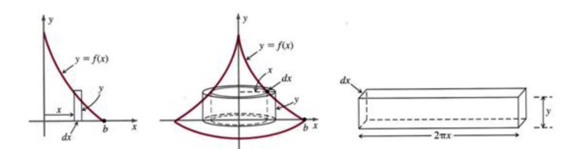
我们可以将其中 \(\mathrm{d}x\) 旋转的图像视作为以 \(y\) 轴为中心，\(x\) 为半径，高度为 \(y\)，厚度为 \(\mathrm{d}x\) 的空心圆柱（展开后为长方体），我们知道空心圆柱体公式为 \(V = 2 \pi r \cdot h \cdot w\)

\[ \mathrm{d}V = 2 \pi r \cdot h \cdot w = 2\pi x \cdot y \cdot \mathrm{d}x \\[1em] V = \int^b_a \mathrm{d}V = 2\pi \int^b_a xf(x)\mathrm{d}x \]

对于参数方程 \(y(t), x(t)\)，则是

\[ \mathrm{d}x = x'(t)\cdot \mathrm{d}t \\[0.6em] V = 2 \pi \int_{a}^{b} x(t)y(t) \cdot x'(t) ~\mathrm{d}t \]

同理我们可以得到绕 \(x\) 轴旋转所形成的体积为

\[V = 2\pi \int^b_a yf^{-1}(y)\mathrm{d}y\]

对于参数方程 \(y(t), x(t)\)，则是

\[ \mathrm{d}y = y'(t)\cdot \mathrm{d}t \\[0.6em] V = 2 \pi \int_{a}^{b} x(t)y(t) \cdot y'(t) ~\mathrm{d}t \]

11.3 Polar Coordinate 极坐标

Polar Coordinate 极坐标

• 定义

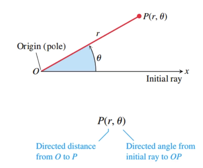
• 极坐标与直角坐标的转换

  • 极转直

  \[\begin{cases} x = r\cos \theta \\ y = r \sin \theta \end{cases}\]

  • 直转极

  \[\begin{cases} r^2 = x^2 + y^2 \\ \tan \theta = \frac{y}{x} \end{cases}\]

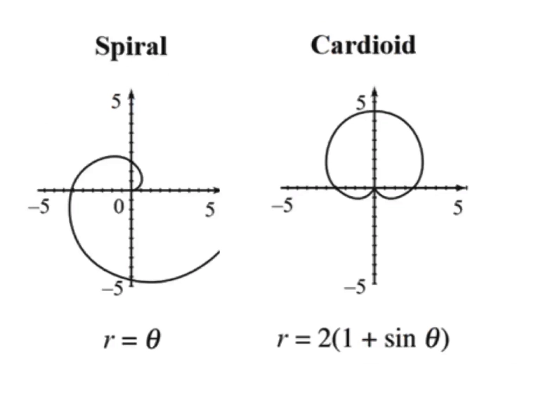
• 对于常见极坐标图像的理解

  • 常用四个点 \(\frac{\pi}{2} \;\; \pi \;\; \frac{3\pi}{2} \;\; 2\pi\) 代入，并给出图像大概的感觉

对于任意极坐标方程都可以通过下列公式转换为直角座标方程

\[ \begin{aligned} &r^{2} = x^{2} + y^{2} & &r = \sqrt{x^{2} + y^{2}} \\[0.8em] &\sin(\theta) = \frac{y}{\sqrt{x^{2} + y^{2}}} & &\cos(\theta) = \frac{x}{\sqrt{x^{2} + y^{2}}} \end{aligned} \]

• 例题

将极坐标方程 \(r^{2} - 8r \sin(\theta) + 12 = 0\) 转换为直角座标方程

\[ \begin{aligned} x^{2} + y^{2} - 8\sqrt{x^{2} + y^{2}} \cdot \frac{y}{\sqrt{x^{2} + y^{2}}} + 12 &= 0 \\ x^{2} + y^{2} -8y + 12 &= 0 \end{aligned} \]

Circle 圆

计算函数 \(r(\theta) = 2a \cos(\theta)\) 所形成圆的半径 \(r\)，和圆心的坐标 \(x, y\)

\[ \begin{aligned} r^{2} &= 2a \cdot (r \cos(\theta)) \\[0.6em] x^{2} + y^{2} &= 2ax \end{aligned} \]

将 \(x^{2} - 2ax\) 配成一个完全平方数，

\[ \begin{aligned} x^{2} - 2ax + a^{2} + y^{2} &= a^{2} \\ (x - a)^{2} + y^{2} &= a^{2} \end{aligned} \]

所以对于函数 \(r(\theta) = 2a \cos(\theta)\) 所形成圆的半径 \(r\)，和圆心的坐标 \(x, y\) 分别为 \(r = a, x = a, y = 0\)

同理，对于 \(r(\theta) = 2a \sin(\theta)\) 所形成圆的半径 \(r\)，和圆心的坐标 \(x, y\) 分别为 \(r = a, x = 0, y = a\)

Tangent Line 切线

给定点 \(P_{0} = (d, \alpha)\)，且点 \(P_{0}\) 是在直线 \(\mathcal{L}\) 上离原点最近的点，求表示 \(\mathcal{L}\) 的极坐标函数

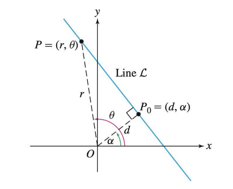
因为 \(P_0\) 在此时为切点，显然 $OP $，所以 \(\triangle OPP_0\) 为直角三角形，所以通过计算 \(\angle POP_{0}\) 的大小（\(\theta - \alpha\)）。所以我们知道了边长 \(OP = d\) 和夹角 \(\angle POP_0\)，通过三角函数 \(\sec(\theta) = \frac{r}{d}\) 得到 \(r\) 关于 \(\theta\) 的表达式如下

\[ \mathcal{L} : r = d \sec(\theta - \alpha) \]

Line 线

对于任意直线 \(\mathcal{L} : y = mx + b\) 都可以表示为

\[ \mathcal{L} : r = \frac{b}{\sin(\theta) - m\cos(\theta)} \]

若将 \(m\) 拆为 \(m = \frac{k}{q}\)，则可表示为

\[ \mathcal{L} : r = \frac{bq}{q\sin(\theta) - k\cos(\theta)} \]

通过下列方式推导

\[ \begin{aligned} \mathcal{L} : y &= \frac{k}{q}x + b \\[0.8em] r \sin(\theta) &= \frac{k}{q} \cdot r \cos(\theta) + b \\[0.8em] r q \sin(\theta) - r k \cos(\theta) &= bq \\[0.8em] \mathcal{L} : r &= \frac{bq}{q \sin(\theta) - k \cos(\theta)} \end{aligned} \]

Derivatives of Polar Coordinate Function 极坐标函数的导数

如果我们有极函数 \(r(\theta)\)，所以每个落在函数上点便可表示为 \((r(\theta), \theta)\)，然后将极坐标函数转化为参数方程

\[ \begin{cases} x = r(\theta)\cos(\theta) \\ y = r(\theta) \sin(\theta) \end{cases} \]

按照参数方程求导公式 \(\frac {dy}{dx} = \frac{y'(t)}{x'(t)}\) 可

\[ \frac{\mathrm{d}y}{\mathrm{d}x} = \frac{\mathrm{d}(r(\theta)\sin(\theta))}{\mathrm{d}(r(\theta)\cos(\theta))} = \frac{r'(\theta)\sin(\theta) + r(\theta)\cos(\theta)}{r'(\theta)\cos(\theta) - r(\theta)\sin(\theta)} \]

11.4 Area and Arc Length of Polar Coordinate Function 极坐标函数的面积与曲线长度

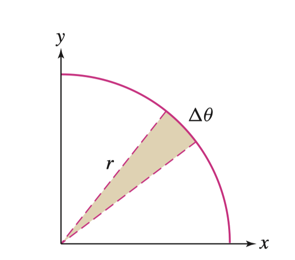
我们通过 \(\mathrm{d}\theta\) 尝试求出每增加 \(\mathrm{d}\theta\) 的角度，算出增量面积，然后将增量面积积起来，即可得到结果。而 \(\mathrm{d}\theta\) 所增量的面积，我们可以近似的看作一个扇形。扇形的面积公式为 \(S_{\text{sector}} = \pi r^2 \cdot \frac{\theta}{2\pi} = \frac{1}{2} r^{2} \theta\)，其中 \(\frac{\theta}{2\pi}\) 便是占整个圆的比值

所以我们可以得到极坐标函数的面积

\[ A=\pi r^2\frac{d\theta}{2\pi}=\int_a^b\frac12 r^2(\theta)d\theta \]

同理我们可以得到两个函数 \(r = f_1(\theta), r = f_2(\theta)\) 相间的面积，其中 \(f_2(\theta) \geqslant f_1(\theta)\)

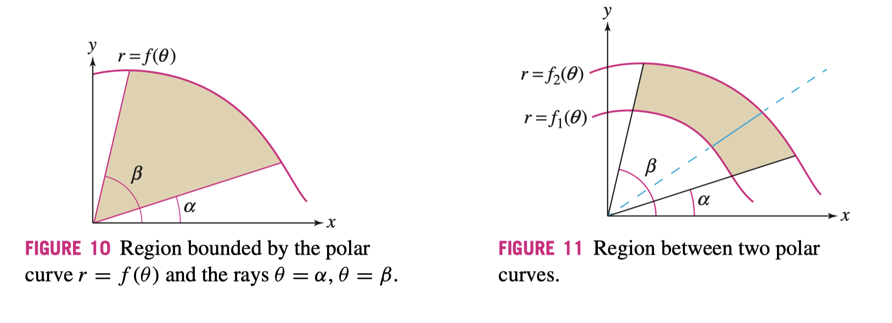
\[ A = \frac{1}{2} \int_{\alpha}^{\beta} (f_{2}(\theta)^{2} - f_{1}(\theta)^{2}) ~\mathrm{d}\theta \]

相似地，极坐标函数的曲线长度和参数方程几乎一样，我们知道参数方程的 \(\mathrm{d}s = \sqrt{x'(t)^{2} + y'(t)^{2}} \cdot \mathrm{d}t\)，所以对于极坐标函数而言

\[ \begin{aligned} x'(\theta) &= \frac{\mathrm{d}x}{\mathrm{d}\theta} = f(\theta) \cos(\theta) = f'(\theta) \cos(\theta) - f(\theta) \sin(\theta) \\[0.8em] y'(\theta) &= \frac{\mathrm{d}y}{\mathrm{d}\theta} = f(\theta) \sin(\theta) = f'(\theta) \sin(\theta) + f(\theta) \cos(\theta) \end{aligned} \]

为了让形式简化看上去更简单，令 \(m = f'(\theta), p = \cos(\theta), n = f(\theta), q = \sin(\theta)\)，其中因为 \(\sin^{2}(x) + \cos^{2}(x) = 1\) 所以 \(q^{2} + p^{2} = 1\)

计算 \(x'(\theta)^{2},\; y'(\theta)^{2}\)

\[ \begin{aligned} x'(\theta)^{2} &= m^{2}p^{2} + n^{2}q^{2} - 2mpnq \\ y'(\theta)^{2} &= m^{2}q^{2} + n^{2}p^{2} + 2mpnq \end{aligned} \]

所以让两式相加并开根号，得到最终形式

\[ \begin{aligned} \sqrt{x'(\theta)^{2} + y'(\theta)^{2}} &= \sqrt{m^{2}p^{2} + n^{2}q^{2} - 2mpnq + m^{2}q^{2} + n^{2}p^{2} + 2mpnq} \\ &= \sqrt{m^{2}(p^{2} + q^{2}) + n^{2}(p^{2} + q^{2})} \\ &= \sqrt{m^{2} + n^{2}} = \sqrt{f'(\theta)^{2} + f(\theta)^{2}} \end{aligned} \]

最后积分得到

\[ S = \int_{a}^{b} \sqrt{(f(\theta))^2 + (f'(\theta))^2} \mathrm{d}\theta \]

• 例题

\(\text{(1)}\) 极函数 \(r^{2}(\theta) = 16 \cos(2\theta)\) 如图所示，计算出其中一个叶子（One Loop）的面积。

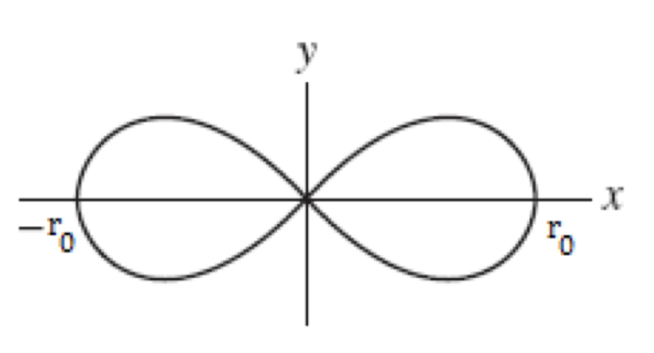
确定半片叶子（Half Loop）的积分上下界，\(r_0\) 时显然 \(\theta = 0\)，原点时也就是使得 \(0 = 16\cos(2\theta)\) 成立（取从 \(0\) 开始第一个成立的解），也就是 \(\theta = \frac{1}{4} \pi\)

\[ 2 \cdot \frac{1}{2} \int_{0}^{\frac{1}{4}\pi} 16 \cos(2\theta) ~\mathrm{d}\theta \]

\(\text{(2)}\) 计算极函数 \(r = \theta^{2}, \theta = 0 \to 4\) 的曲线长度

代入弧长公式

\[ S = \int_{a}^{b} \sqrt{(f(\theta))^2 + (f'(\theta))^2} \mathrm{d}\theta = \int_{0}^{4} \sqrt{(\theta^{2})^{2} + (2\theta)^{2}} ~\mathrm{d}\theta = \frac{8}{3}\left(5\sqrt{5} - 1\right) \]

11.5 Conic Section 圆锥曲线

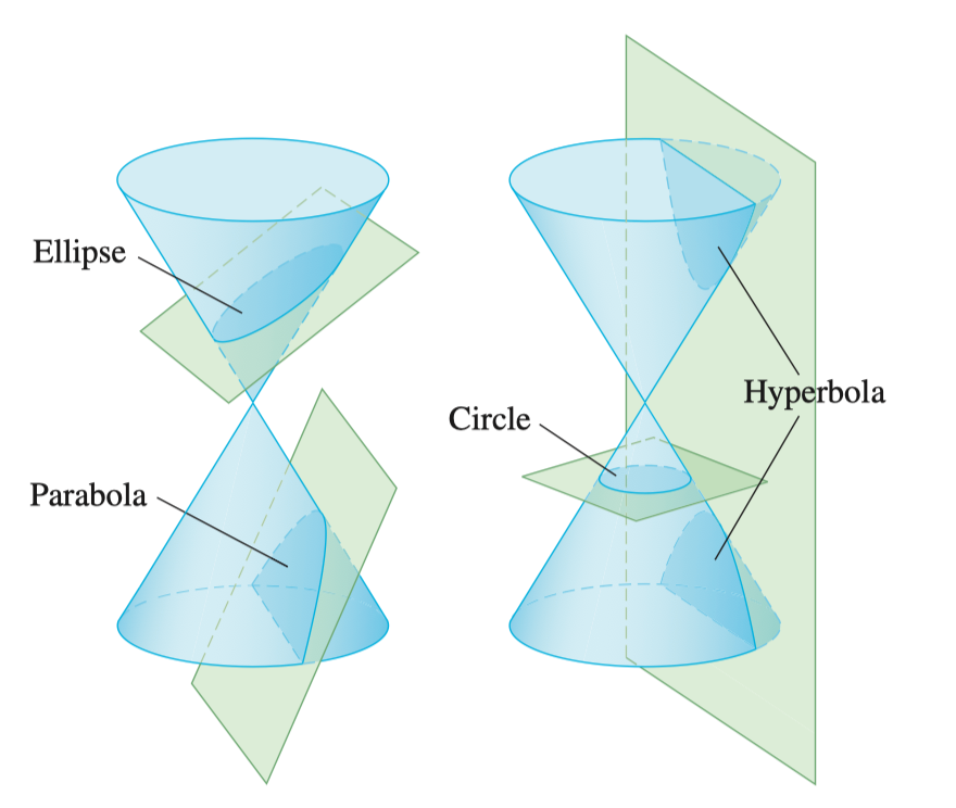
Ellipse 椭圆

椭圆的几何定义为，若存在点 \(F_1, F_2, P\) 满足下列关系，\(P\) 的轨迹则为椭圆（如下图所示）

\[ PF_1 + PF_2 = K \]

其中，点 \(F_1, F_2\) 为焦点（Foci, Focus for plural），如果将焦点拉至重合，原关系则为 \(2PF = K\) 椭圆将会退化为半径为 \(\frac{1}{2} K\) 的圆形，中心为 \(F_1\) 或 \(F_2\)

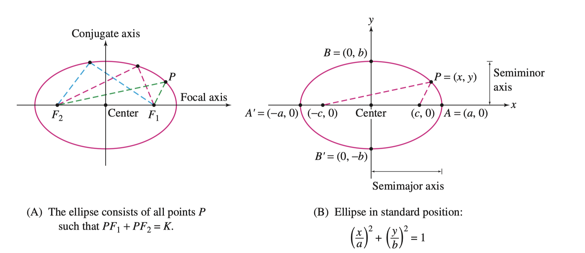
我们定义：

• \(\overline{F_1F_2}\) 的中点为椭圆的中心（Center of the Ellipse）
• 焦点所在的数轴为焦轴（Focal Axis），与之垂直的数轴为共轭轴（Conjugate Axis）
  • 如果是图中的焦轴，写作横焦轴（Horizontal Focal Axis），旋转 \(90^\circ\) 为竖焦轴（Vertical Focal Axis）
• 其中还有半长轴（Semimajor Axis），和半短轴（Semiminor Axis），如图上右图所示

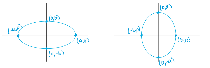
当 \(a \geqslant b > 0\) 椭圆的标准参数方程为 \[ \frac{x^{2}}{a^{2}} + \frac{y^{2}}{b^{2}} = 1 \quad\quad\quad\quad\quad \frac{x^{2}}{b^{2}} + \frac{y^{2}}{a^{2}} = 1 \]

其中 \(a = \frac{K}{2}\), \(b = \sqrt{a^{2} - c^{2}}\)

具体的证明见下图（其实这个过程了解一下就可以）

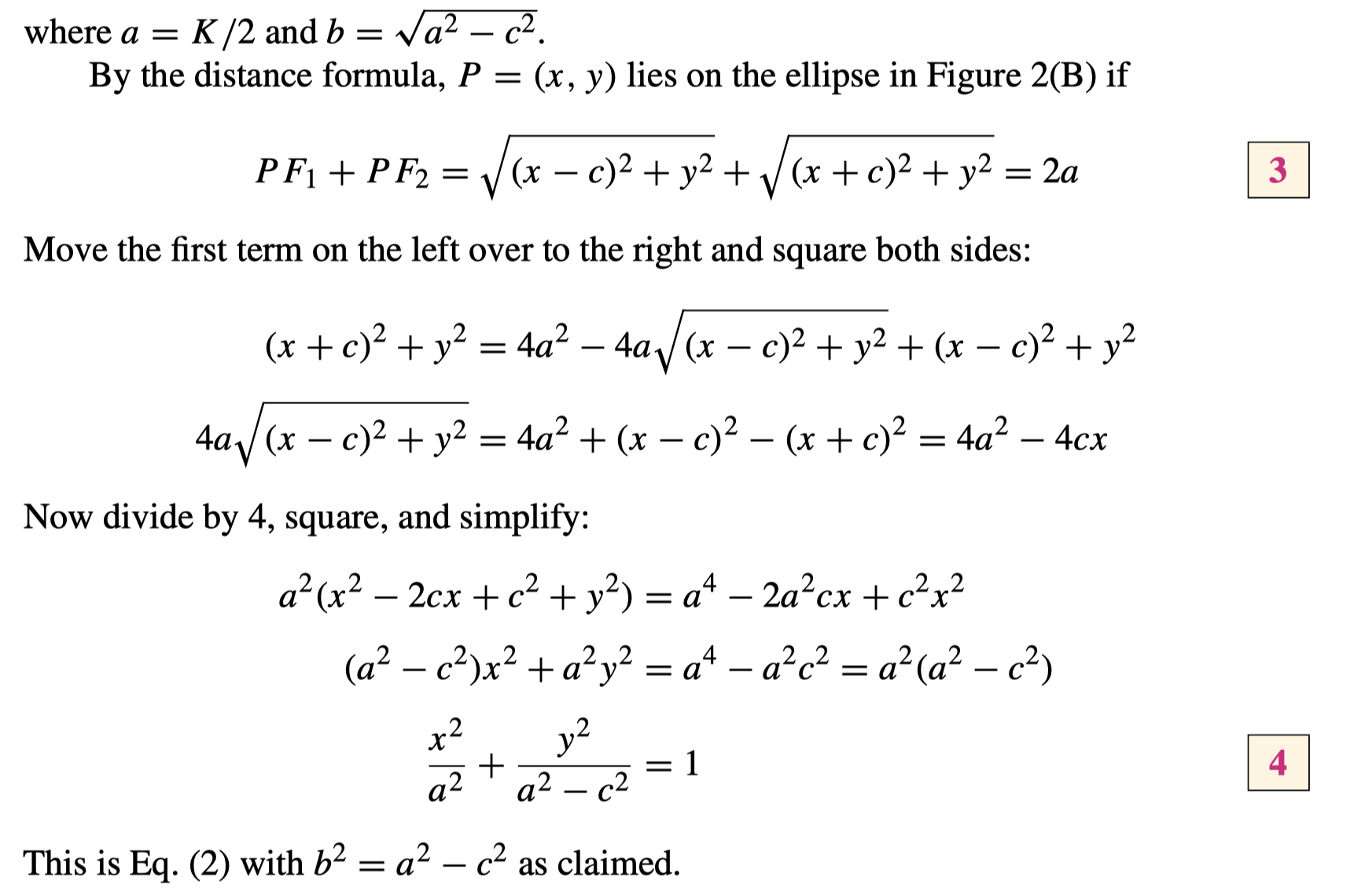
椭圆标准方程的平移和圆标准方程的平移非常相似，若圆心为 \(C = (h, k)\)，则有

\[ \left(\frac{x - h}{a}\right)^{2} + \left(\frac{y - k}{b}\right)^{2} = 1 \]

Hyperbola 双曲线

双曲线的几何定义为，若存在点 \(F_1, F_2, P\) 满足下列关系，\(P\) 的轨迹则为双曲线（如下图所示），其中 \(\pm K\) 的来源就是为了满足 \(P\) 和 \(Q\) 点两种形式

\[ PF_1 - PF_2 = \pm K \]

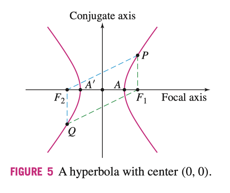
我们定义：

• \(\overline{F_1F_2}\) 的中点为双曲线的中心（Center of the Hyperbola）
• 焦点所在的数轴为焦轴（Focal Axis），与之垂直的数轴为共轭轴（Conjugate Axis）
  • 如果是图中的焦轴，写作横焦轴（Horizontal Focal Axis），旋转 \(90^\circ\) 为竖焦轴（Vertical Focal Axis）
• 我们将图中的 \(a\) 称之为实半轴，\(b\) 称之为虚半轴

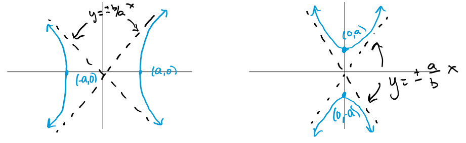
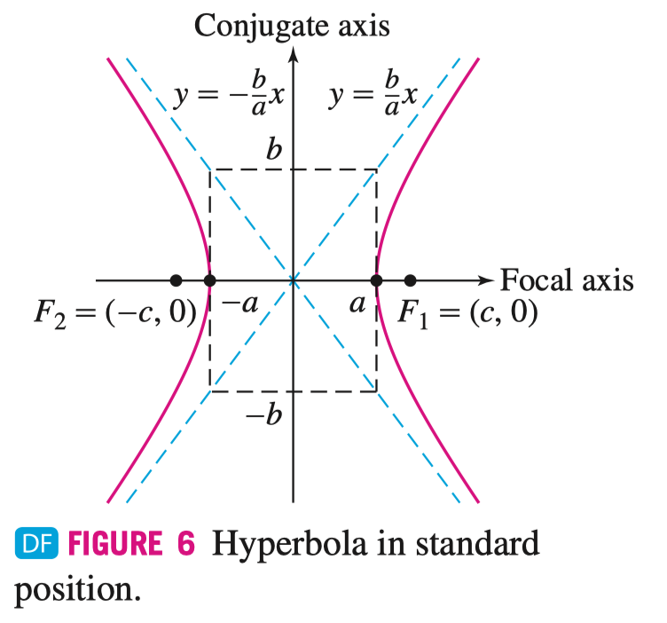
当 \(a \geqslant b > 0\) 双曲线的标准参数方程为

\[ \begin{aligned} \text{Equation:}& & &\frac{x^{2}}{a^{2}} - \frac{y^{2}}{b^{2}} = 1 & &\frac{y^{2}}{a^{2}} - \frac{x^{2}}{b^{2}} = 1 \\ \text{Asymptotes:}& & &y = \pm \frac{b}{a} x & &y = \pm \frac{a}{b}x \end{aligned} \]

其中 \(2a = \pm K\), \(c = \sqrt{a^{2} + b^{2}}\)

摆烂了，后面不证了，读者自证不难（逃

Parabola 抛物线

抛物线的几何定义为，若存在点 \(F, P\) 和直线 $ $ 满足如下关系，\(P\) 的轨迹则为抛物线（如下图所示），其中直线 \(\mathcal{D} : y = -c\)，我们称之为准线（Directrix），焦点 \(F = (0, c)\)

\[ PF = P\mathcal{D} \]

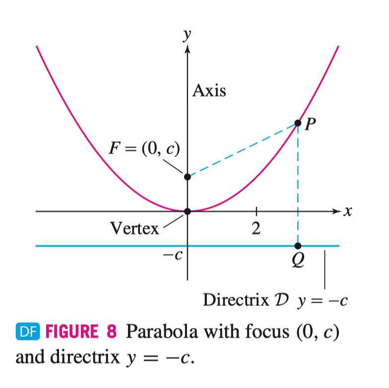
抛物线的标准参数方程是

\[ y = \frac{1}{4c} x^{2} \]

其中，若 \(c > 0\) 开口向上，\(c < 0\) 则开口向下

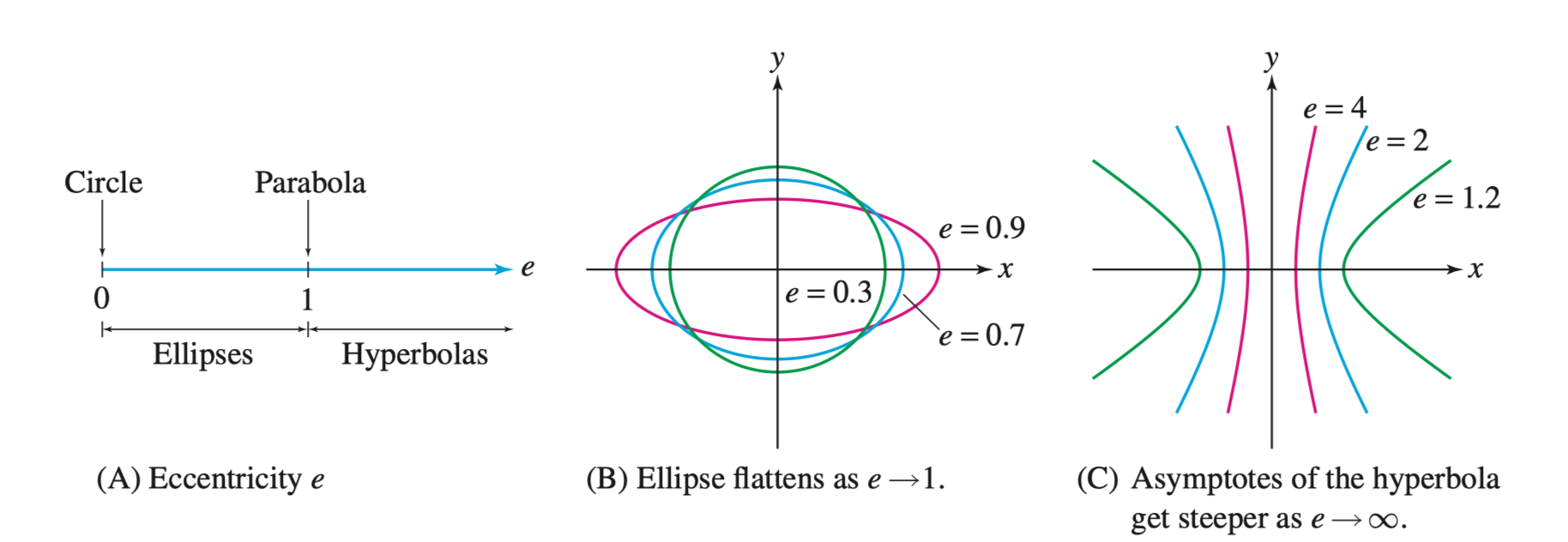
Eccentricity 离心率

离心率（Eccentricity）\(e\) 的定义为，焦点之间距离与焦轴上点的距离之比，也就是 \(e = \frac{c}{a}\)

• 离心率在 \(0 \leqslant e < 1\) 时，为椭圆
• 离心率在 \(e > 1\) 时，为双曲线

离心率可以用于统一圆锥曲线的几何定义

\[ PF = eP \mathcal{D} \]

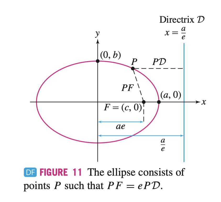
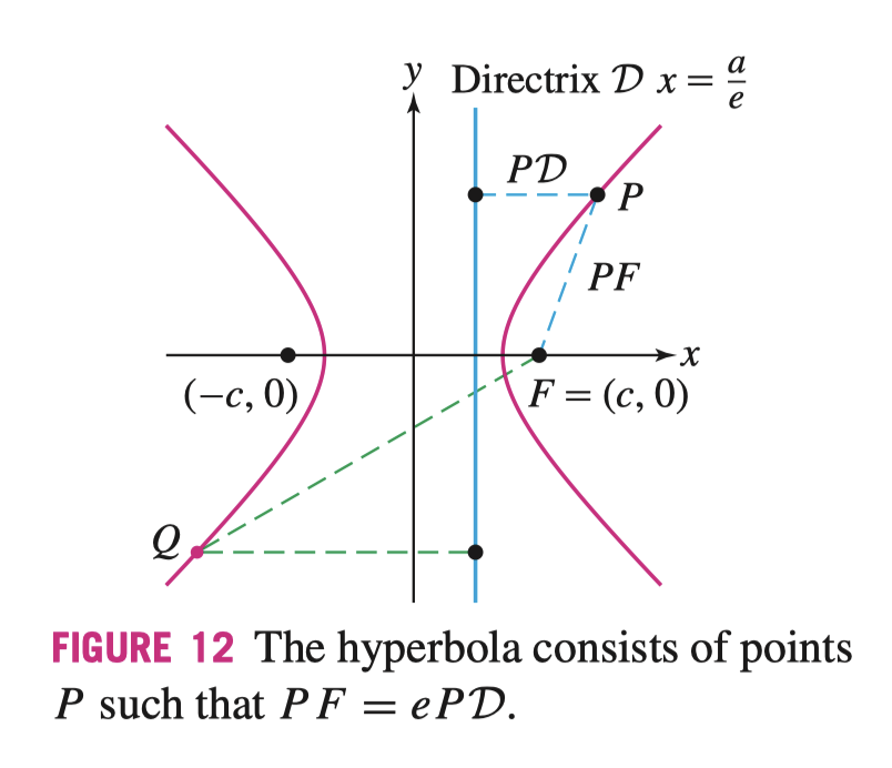
椭圆和双曲线的准线均为 \(x = \frac{a}{e}\)

对于圆锥曲线离心率 \(e > 0\)，并且焦点在原点，且准线 \(x = d\) 时的极坐标函数表达为 \[ r = \frac{ed}{1 + e \cos (\theta)} \]

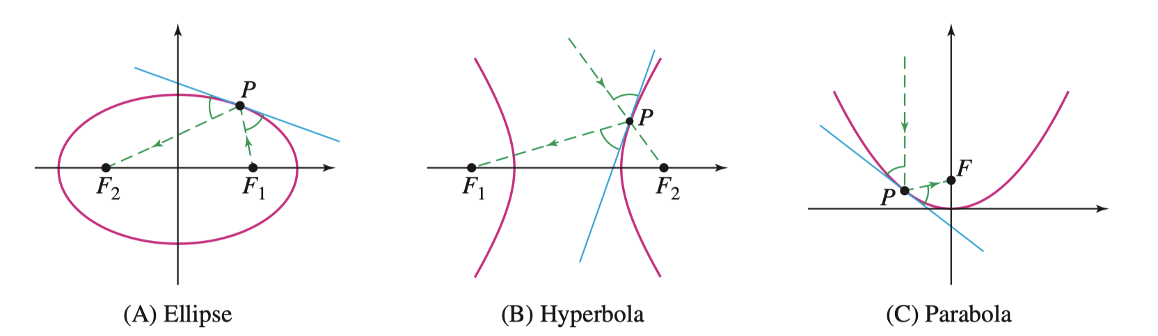
Reflective Properties of Conic Sections 圆锥曲线的反射性

General Equations of Degree 2 二阶圆锥曲线的通用公式

对于任何二阶圆锥曲线都可以通过以下的一般公式表示

\[ ax^{2} + bxy + cy^{2} + dx + ey + f = 0 \]

并且可以表示圆锥曲线的非标准形式，比如焦轴并不是 \(90^\circ\)，如图所示

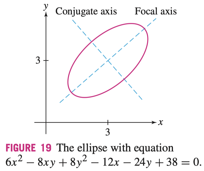
如果上式的解为相交线，平行线，一条直线，一个点，或者是空集，我们便说这个等式退化（Degenerate）了，例如：

• \(x^{2} - y^{2} = 0\) 定义了一组相交线 \(y = x, y = -x\)
• \(x^{2} - x = 0\) 定义了一组平行线 \(x = 0, x = 1\)
• \(x^{2} = 0\) 定义了一条直线（\(y\) 轴）
• \(x^{2} + y^{2} = 0\) 只有一个解 \((0, 0)\)
• \(x^{2} + y^{2} = -1\) 没有解

在这个通用公式中，\(bxy\) 项称为交叉项（Cross Term），如果其为 \(0\)，则可以被表示为标准形式（即不旋转焦轴）

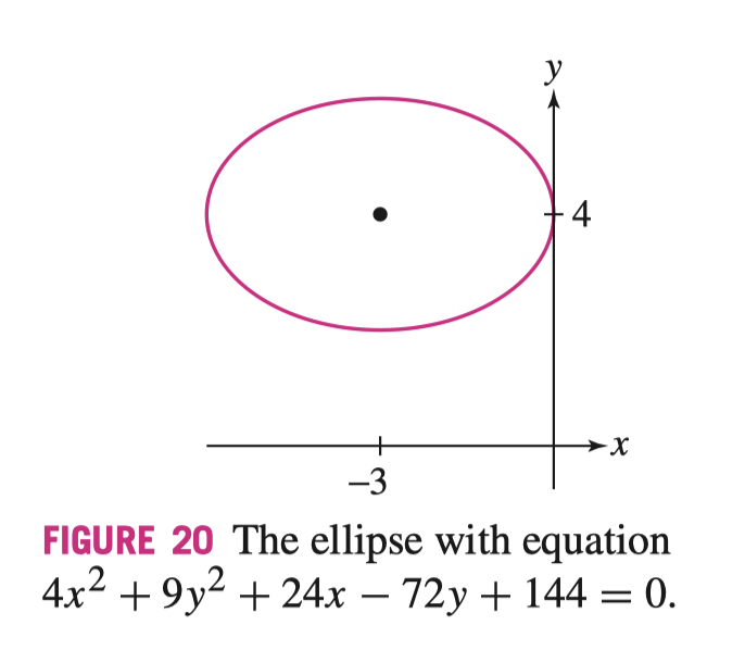
比如对于 \(4x^{2} + 9y^{2} + 24x - 72y + 144 = 0\) 就可以化为 \(4(x + 3)^{2} + 9(y - 4)^{2} = 36\)，进而化为椭圆标准方程

\[ \left(\frac{x+3}{3}\right)^{2} + \left(\frac{y-4}{2}\right)^{2} = 1 \]

我们可以将通过判别式（Discriminant）判断通用式中圆锥曲线的形状

\[ D = b^{2} - 4ac \]

判别式有以下几种情况： - \(D < 0\): 椭圆或者圆 - \(D > 0\): 双曲线 - \(D = 0\): 抛物线

12 Vector Geometry 向量几何

12.1-12.5 Vectors in the Plane 向量

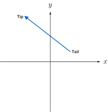
向量（Vector）的几何意义就是从尾（Tail）指到头（Tip）的一个箭头，代数意义为从原点出发指向坐标 \(\left<a, b \right>\) 的箭头。

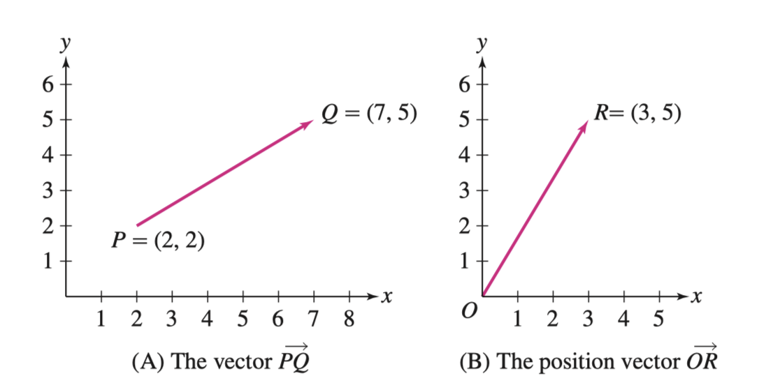
对于向量 \(\mathbf{v} = \overrightarrow{PQ}\) 向量的长度（Length）或者说大小（Magnitude）写作 \(\left\| \mathbf{v} \right\|\)，表示从 \(P\) 到 \(Q\) 的距离，通过勾股定理，很容易得到

\[ \left\| \mathbf{v} \right\| = \sqrt{(x_1 - x_2)^{2} + (y_1 - y_2)^{2}} \]

Vector Algebra 向量代数

如下图所示，向量的几何加减法遵循平行四边形法则（Parallelogram Law），若是减法，则反转被减向量的方向，然后按照同样的规则进行加法

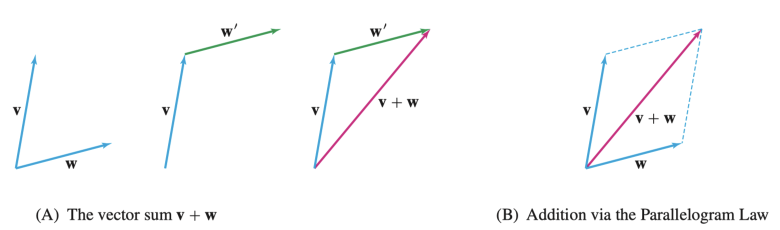
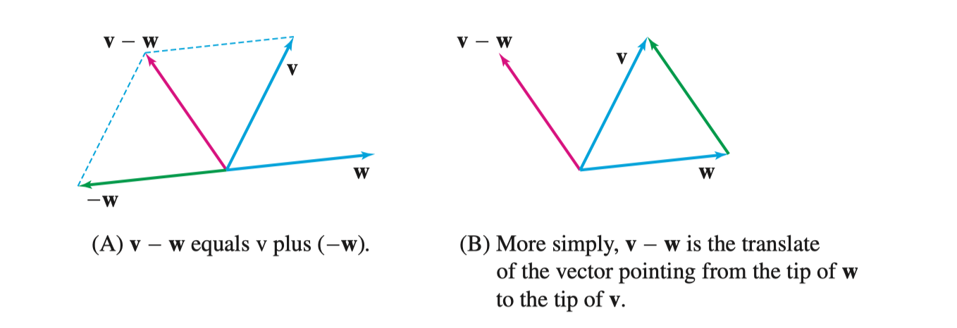
Shortcut: \(\mathbf{A} - \mathbf{B}\) 是从 \(\mathbf{B}\) 出发指向 \(\mathbf{A}\) 的向量，谁被减从谁出发

其代数表示则为，\(\mathbf{v}\mapsto\left< a, b \right> + \mathbf{w}\mapsto\left< c, d \right> = \left< a + c, b + d \right>\)

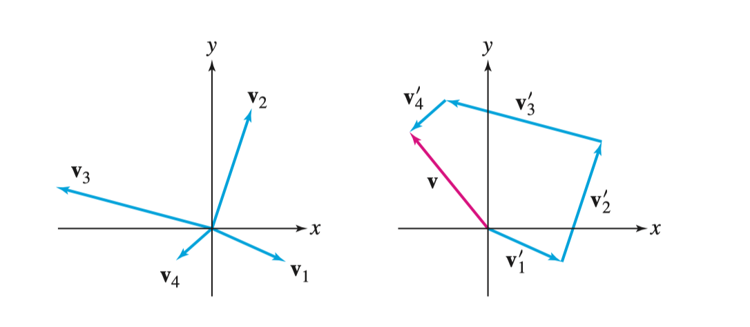
对于多个向量的加法如图所示（这一性质使得向量可以非常轻松的构造复杂运动的参数方程）

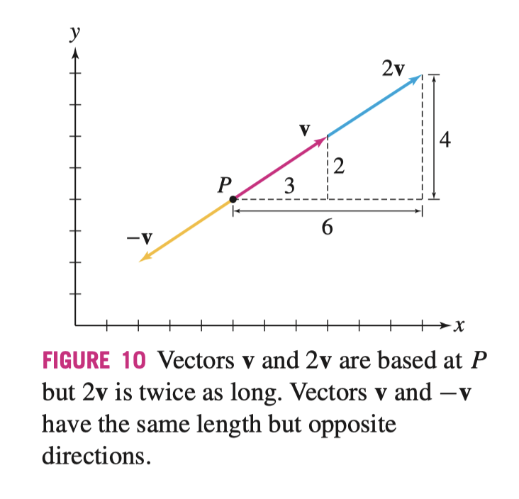
向量与标量（Scalar）的乘法（Scalar Multiple）\(c \mathbf{v} = \left< cv_1, cv_2, \cdots ,cv_n \right>\)，且 \(\| c \mathbf{v} \| = |c| \| \mathbf{v} \|\)

从几何意义上来说，标量乘法是成倍数的放大原有向量，如下图所示

向量运算遵循下列基本性质

\[ \begin{aligned} &\mathbf{v} + \mathbf{w} = \mathbf{w} + \mathbf{v} & &\text{Commutative Law} \\ &\mathbf{u} + (\mathbf{v} + \mathbf{w}) = (\mathbf{u} + \mathbf{v}) + \mathbf{w} & &\text{Associative Law}\\ &c(\mathbf{v} + \mathbf{w}) = c \mathbf{v} + c \mathbf{w} & &\text{Distributive Law for Scalars} \\ \end{aligned} \]

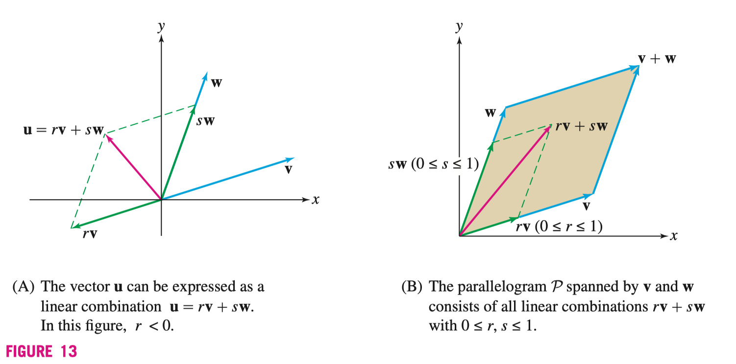
线性组合（Linear Combination）是多个非平行向量与其对应标量相加，例如，向量 \(\mathbf{v}, \mathbf{w}\) 的线性组合为

\[ r \mathbf{v} + s \mathbf{w} \]

在 \(\mathbf{v}, \mathbf{w}\) 的平面上，任何向量都可以被表示为 \(\mathbf{u} = r \mathbf{v} + s \mathbf{w}\)，若 \(0 \leqslant r, s \leqslant 1\) 则包含 \(\mathbf{v}, \mathbf{w}\) 所形成平行四边形内的所有点

若一个向量的单位长度为 \(1\)，则我们称这个向量为单位向量（Unit Vector），单位向量通常用来表示方向，对于任意向量 \(\mathbf{v} = \left<v_1, v_2 \right>\) 我们可以通过标准化（Normalize）获得其单位向量

\[ \hat{\mathbf{v}} = \frac{1}{\|\mathbf{v}\|} \cdot \mathbf{v} = \frac{\mathbf{v}}{\|\mathbf{v}\|} \]

一般的，通过单位向量 \(\hat{\mathbf{e}} = \left<\cos(\theta), \sin(\theta) \right>\)，可以描述 \(\theta\) 角度下的单位向量，所以对于任意向量 \(\mathbf{v}\)

\[ \mathbf{v} = \|\mathbf{v}\| \hat{\mathbf{e}} = \|\mathbf{v}\| \left< \cos(\theta), \sin(\theta) \right> \]

在标准笛卡尔二维坐标系中，我们通常使用标准基向量（Standard Basis Vector） \(\mathbf{i} \mapsto \left<1, 0 \right>, ~ \mathbf{j}\mapsto \left<0, 1 \right>\) 通过线性组合以表示在该平面上的任意一向量。例如，对于向量 \(\mathbf{v}\)

\[ \mathbf{v} \mapsto \left<a, b \right> = a \mathbf{i} + b \mathbf{j} \]

依据三角形不等式，我们可以很容易得出

\[ \| \mathbf{v} + \mathbf{w} \| \leqslant \left\| \mathbf{v} \right\| + \left\| \mathbf{w} \right\| \\ \text{where } \mathbf{v} \neq 0 \]

12.2 Vectors in Three Dimensions 三维向量

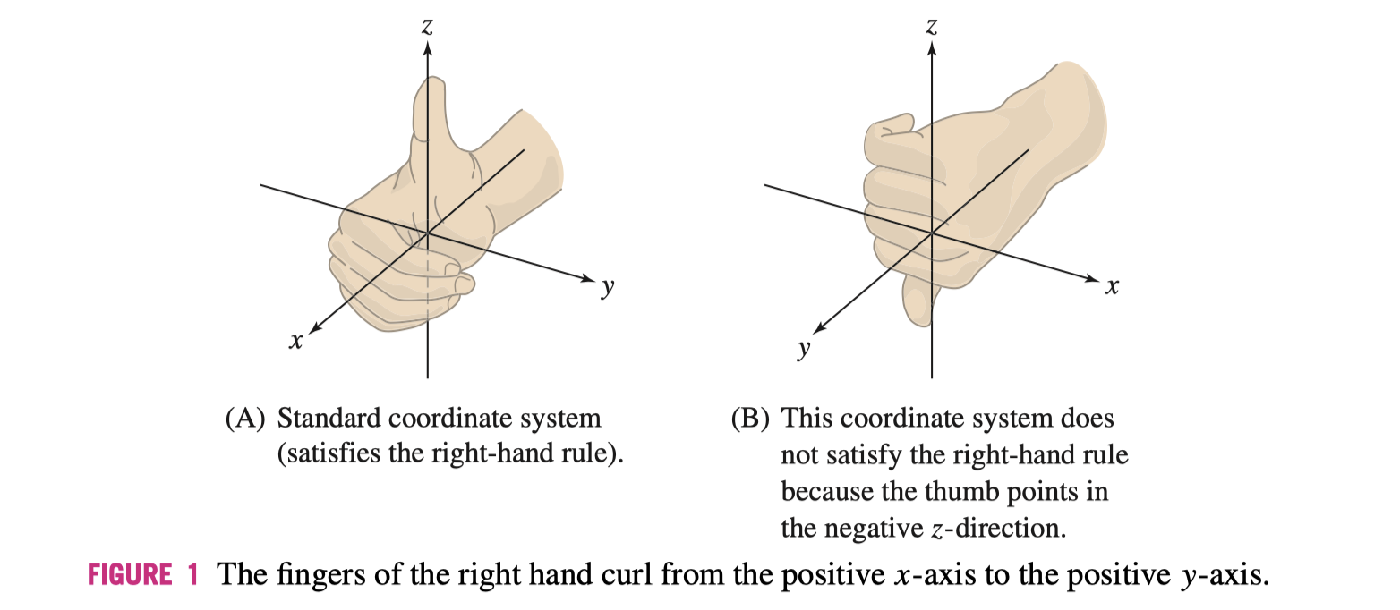
三维坐标系的位置遵循右手定则，即大拇指指向方向为 \(z\) 轴，其他四指指向 \(x\) 轴后握紧。

Sphere 球面

对于任意一个在 \(\mathbb{R}^{3}\) 中心为 \((a, b, c)\) 的圆球

\[ (x - a)^{2} + (y - b)^{2} + (z - c)^{2} = R^{2} \]

Cylinder 圆柱

对于任意一个在 \(\mathbb{R}^{3}\) 中心为 \((a, b, 0)\)

\[ (x - a)^{2} + (y - b)^{2} = R^{2} \]

Equation of a Line (Point-Direction Form) 直线方程与向量

对于穿过点 \(P_0 = (x_0, y_0, z_0)\) ，方向为 \(\mathbf{v} = \left< a, b, c \right>\) 的直线 \(\mathcal{L}\)，可以通过下列方程描述

\[ \mathbf{r}(t) = \mathbf{r}_0 + t \mathbf{v} = \left< x_0, y_0, z_0 \right> + t\left<a, b, c \right> \]

其中 \(\mathbf{r}_0 = \overrightarrow{OP_0}\)

与之对应的参数方程分别为

\[ \begin{cases} x = x_0 + at \\ y = y_0 + bt \\ z = z_0 + ct \end{cases} \]

Dot Product and the Angle Between Two Vectors 点乘与向量夹角

Dot Product 点乘

对于向量 \(\mathbf{A}, \mathbf{B}\) 我们定义点乘（Dot Product）的代数形式如下，其结果为标量（Scalar）

\[ \mathbf{A} \cdot \mathbf{B} = \sum a_i b_i = a_1 b_1 + a_2 b_2 + a_3 b_3 \]

其几何形式的定义为

\[ \mathbf{A} \cdot \mathbf{B} = \left\| \mathbf{A} \right\| \left\|\mathbf{B}\right\| \cos(\theta) \]

两个定义可以通过余弦定理进行统一，以后补上

所以我们可以通过向量获得夹角

\[ \cos(\theta) = \frac{\mathbf{A} \cdot \mathbf{B}}{\left\| \mathbf{A} \right\| \left\| \mathbf{B} \right\|} \]

也可以通过这一性质来判断夹角的性质

\[ \begin{cases} \cos(\theta) > 0 & \theta < \frac{\pi}{2}\\ \cos(\theta) < 0 & \theta > \frac{\pi}{2}\\ \cos(\theta) = 0 & \perp \end{cases} \implies \begin{cases} \text{Dot Product} > 0 & \theta \text{ is acute}\\ \text{Dot Product} < 0& \theta \text{ is obtuse}\\ \text{Dot Product} = 0& \perp, 90^\circ \end{cases} \]

Properties of Dot Product 点乘的性质

\[ \begin{aligned} &0 \cdot \mathbf{v} = \mathbf{v} \cdot 0 = 0 & & \\ &\mathbf{v} \cdot \mathbf{w} = \mathbf{w} \cdot \mathbf{v} & &\text{Commutativity} \\ &(c \mathbf{v}) \cdot \mathbf{w} = \mathbf{v} \cdot (c \mathbf{w}) = c (\mathbf{v} \cdot \mathbf{w}) & &\text{Pulling out Scalars}\\ & \mathbf{u} \cdot (\mathbf{v} + \mathbf{w}) = \mathbf{u} \cdot \mathbf{v} + \mathbf{u} \cdot \mathbf{w} & &\text{Distributive Law} \\ & \mathbf{v} \cdot \mathbf{v} = \| \mathbf{v} \|^{2} & &\text{Relation with Length} \end{aligned} \]

Projection of Vectors 向量的投影

若 \(\mathbf{v} \neq 0\)，则我们定义 \(\mathbf{u}\) 在 \(\mathbf{v}\) 上的投影（Projection）是 \(\mathbf{u}_{\parallel \mathbf{v}}\) 或者 \(\operatorname{proj}_{\mathbf{v}} \mathbf{u}\)

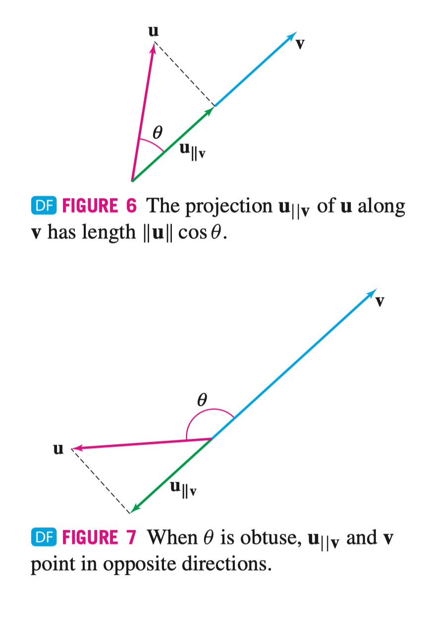
\[ \begin{aligned} \mathbf{u}_{\parallel \mathbf{v}} = \|\mathbf{u}\| \cos(\theta) \hat{\mathbf{e}_{\mathbf{v}}} &= \|\mathbf{u}\| \left(\frac{\mathbf{u} \cdot \mathbf{v}}{\|\mathbf{u}\| \|\mathbf{v}\|}\right) \cdot \frac{\mathbf{v}}{\|\mathbf{v}\|} \\[0.8em] &= \left(\frac{\mathbf{u} \cdot \mathbf{v}}{\|\mathbf{v}\|^{2}}\right) \mathbf{v} \\[0.8em] &= \left(\frac{\mathbf{u} \cdot \mathbf{v}}{\mathbf{v} \cdot \mathbf{v}}\right) \mathbf{v} \\[0.8em] &= \left(\frac{\mathbf{u} \cdot \mathbf{v}}{\|\mathbf{v}\|}\right) \hat{\mathbf{e}_{\mathbf{v}}} \end{aligned} \]

其中 \(\frac{\mathbf{u} \cdot \mathbf{v}}{\|\mathbf{v}\|}\) 称为 \(\mathbf{u}\) 在 \(\mathbf{v}\) 上投影的标量因子（Scalar Component）表示为 \(\operatorname{comp}_{\mathbf{v}} \mathbf{u}\)

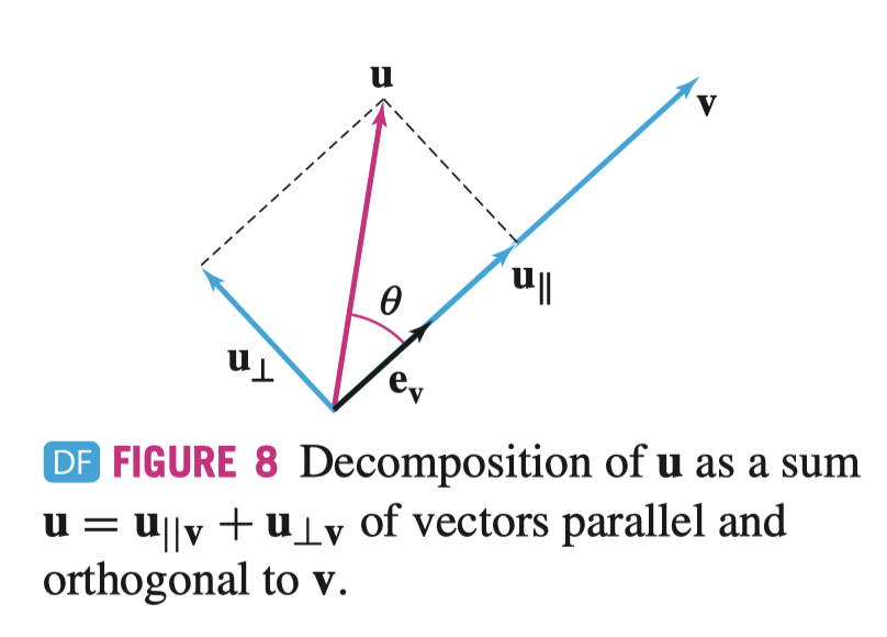
我们还可以通过正交分解向量 \(\mathbf{u}\) 定义 \(\mathbf{u}_{\perp \mathbf{v}}\) 如下

\[ \mathbf{u} = \mathbf{u}_{\parallel \mathbf{v}} + \mathbf{u}_{\perp \mathbf{v}} \]

12.4 The Cross Product 叉乘

\(2 \times 2\) 行列式（Determinants）

\[ \begin{vmatrix} a_{11} & a_{12} \\a_{21} & a_{22} \\ \end{vmatrix} = a_{11} a_{22} - a_{12} a_{21} \]

\(3 \times 3\) 行列式

\[ \begin{vmatrix} a_{11} & a_{12} & a_{13} \\ a_{21} & a_{22} & a_{23} \\ a_{31} & a_{32} & a_{33} \\ \end{vmatrix} = a_{11} \begin{vmatrix} a_{22} & a_{23} \\ a_{32} & a_{33} \\ \end{vmatrix} - a_{12} \begin{vmatrix} a_{21} & a_{23} \\ a_{31} & a_{33} \\ \end{vmatrix} + a_{13} \begin{vmatrix} a_{21} & a_{22} \\ a_{31} & a_{32} \\ \end{vmatrix} \]

我们定义 \(\mathbf{v} = \left< v_1, v_2, v_3 \right>\)，和 \(\mathbf{w} = \left<w_1, w_2, w_3 \right>\) 的叉乘（Cross Product）为

\[ \mathbf{v} \times \mathbf{w} = \begin{vmatrix} \mathbf{i} & \mathbf{j} & \mathbf{k} \\ v_1 & v_2 & v_3 \\ w_1 & w_2 & w_3 \\ \end{vmatrix} = \begin{vmatrix} v_2 & v_3 \\ w_2 & w_3 \\ \end{vmatrix} \mathbf{i} - \begin{vmatrix} v_1 & v_3 \\ w_1 & w_3 \\ \end{vmatrix} \mathbf{j} + \begin{vmatrix} v_1 & v_2 \\ v_1 & v_2 \\ \end{vmatrix} \mathbf{k} \]

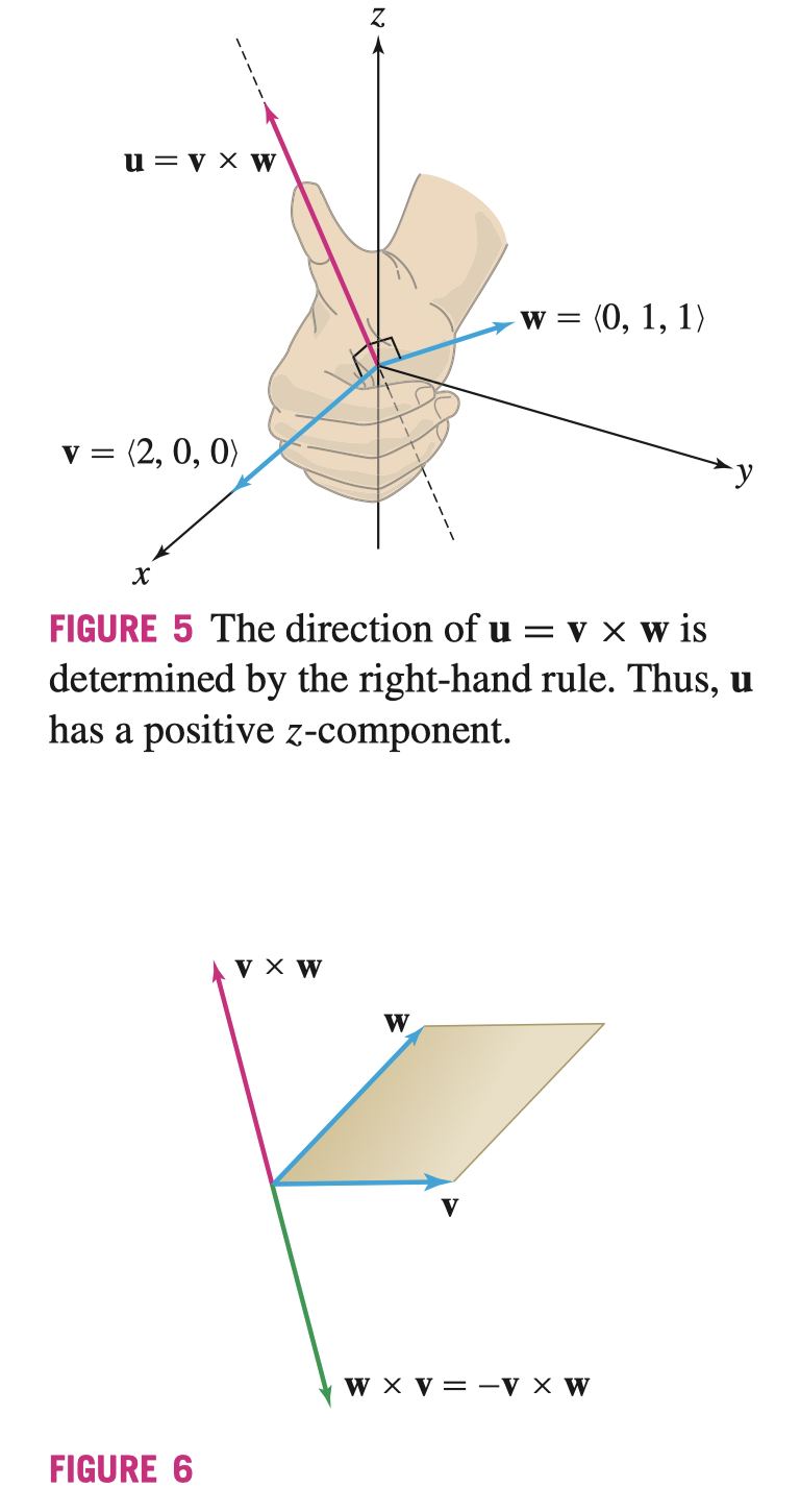
叉乘 \(\mathbf{v} \times \mathbf{w}\) 的结果是向量，并且有如下性质

• \(\mathbf{v} \times \mathbf{w}\) 正交于 \(\mathbf{v}\) 和 \(\mathbf{w}\)
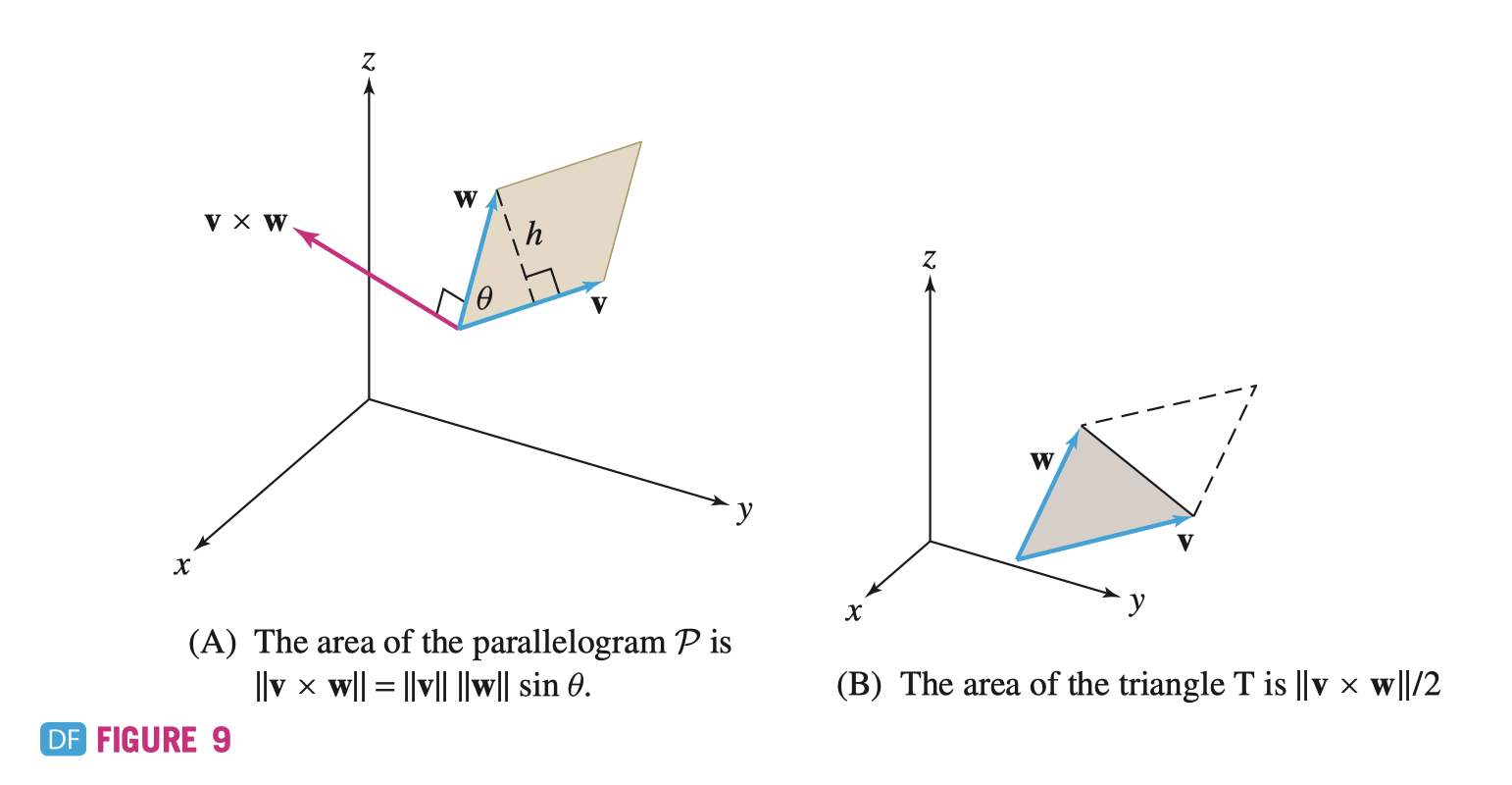
• \(\mathbf{v} \times \mathbf{w}\) 的长度为 \(\|\mathbf{v}\| \| \mathbf{w} \| \sin(\theta)\)，\(\theta\) 为 \(\mathbf{v}\) \(\mathbf{w}\) 之间的夹角，且 $0 $
• \({\mathbf{v}, \mathbf{w}, \mathbf{v} \times \mathbf{w}}\) 符合右手定则
• \(\mathbf{w} \times \mathbf{v} = -\mathbf{v} \times \mathbf{w}\)
• \(\mathbf{v} \times \mathbf{w} = 0\) 当且仅当 \(\mathbf{w} = c \mathbf{v}\)（\(\mathbf{w}, \mathbf{v}\) 共线），或者 \(\mathbf{v} = 0\)
• \((c \mathbf{v}) \times \mathbf{w} = \mathbf{v} \times (c \mathbf{w}) = c(\mathbf{v} \times \mathbf{w})\)
• \((\mathbf{u} + \mathbf{v}) \times \mathbf{w} = \mathbf{u} \times \mathbf{w} + \mathbf{v} \times \mathbf{w}\) （交换律较为特殊，注意乘法顺序）
• \(\mathbf{v} \times (\mathbf{u} + \mathbf{w}) = \mathbf{v} \times \mathbf{u} + \mathbf{v} \times \mathbf{w}\) （交换律较为特殊，注意乘法顺序）

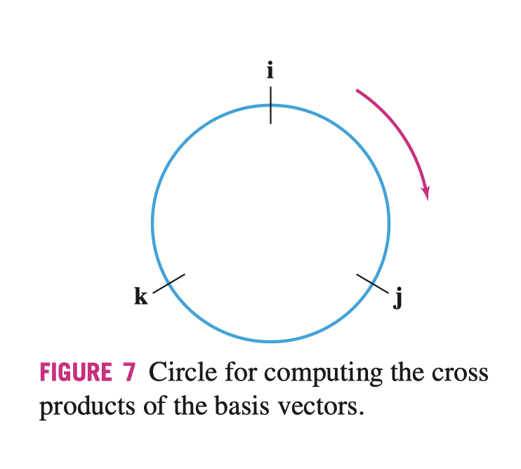
基向量 \(\mathbf{i}, \mathbf{j}, \mathbf{k}\) 的轮转

\[ \mathbf{i} \times \mathbf{j} = \mathbf{k} \quad \mathbf{j} \times \mathbf{k} = \mathbf{i} \quad \mathbf{k} \times \mathbf{i} = \mathbf{j} \]

\(\| \mathbf{v} \times \mathbf{w} \|\) 为对于平行四边形的面积，\(\frac{1}{2} \| \mathbf{v} \times \mathbf{w} \|\) 为对应三角形的面积

对于叉乘，我们有以下恒等式

\[ \| \mathbf{v} \times \mathbf{w} \|^{2} = \| \mathbf{v} \|^{2} \| \mathbf{w} \|^{2} - (\mathbf{v} \cdot \mathbf{w})^{2} \]

定义三矢量积（Vector Triple Product）为 \(\mathbf{u} \cdot (\mathbf{v} \times \mathbf{w})\)（其结果为标量）我们有

\[ \mathbf{u} \cdot (\mathbf{v} \times \mathbf{w}) = \operatorname{det} \begin{pmatrix} \mathbf{u} \\ \mathbf{v} \\ \mathbf{w} \\ \end{pmatrix} \]

\(\mathbf{u}, \mathbf{v}, \mathbf{w}\) 所构成的平行四边体的体积为对应三矢量积 \(| \mathbf{u} \cdot (\mathbf{v} \times \mathbf{w}) |\)

12.5 Planes in 3-Space 三维空间中的平面方程

对于经过点 \(P_0 = \left< x_0, y_0, z_0 \right>\) 平面 $ $ 有法向量 \(\mathbf{n} = \left<a, b, c \right>\)

\[ \begin{aligned} \mathcal{P} : ~&\mathbf{n} \cdot \left< x, y, z \right> &= d \\ \mathcal{P} : ~&a(x - x_0) + b(y - y_0) + c(z - z_0) &= 0 \\ ~&ax + by + cz &= d \end{aligned} \]

其中 \(d = \mathbf{n} \cdot \left<x_0, y_0, z_0 \right> = ax_0 + by_0 + cz_0\)

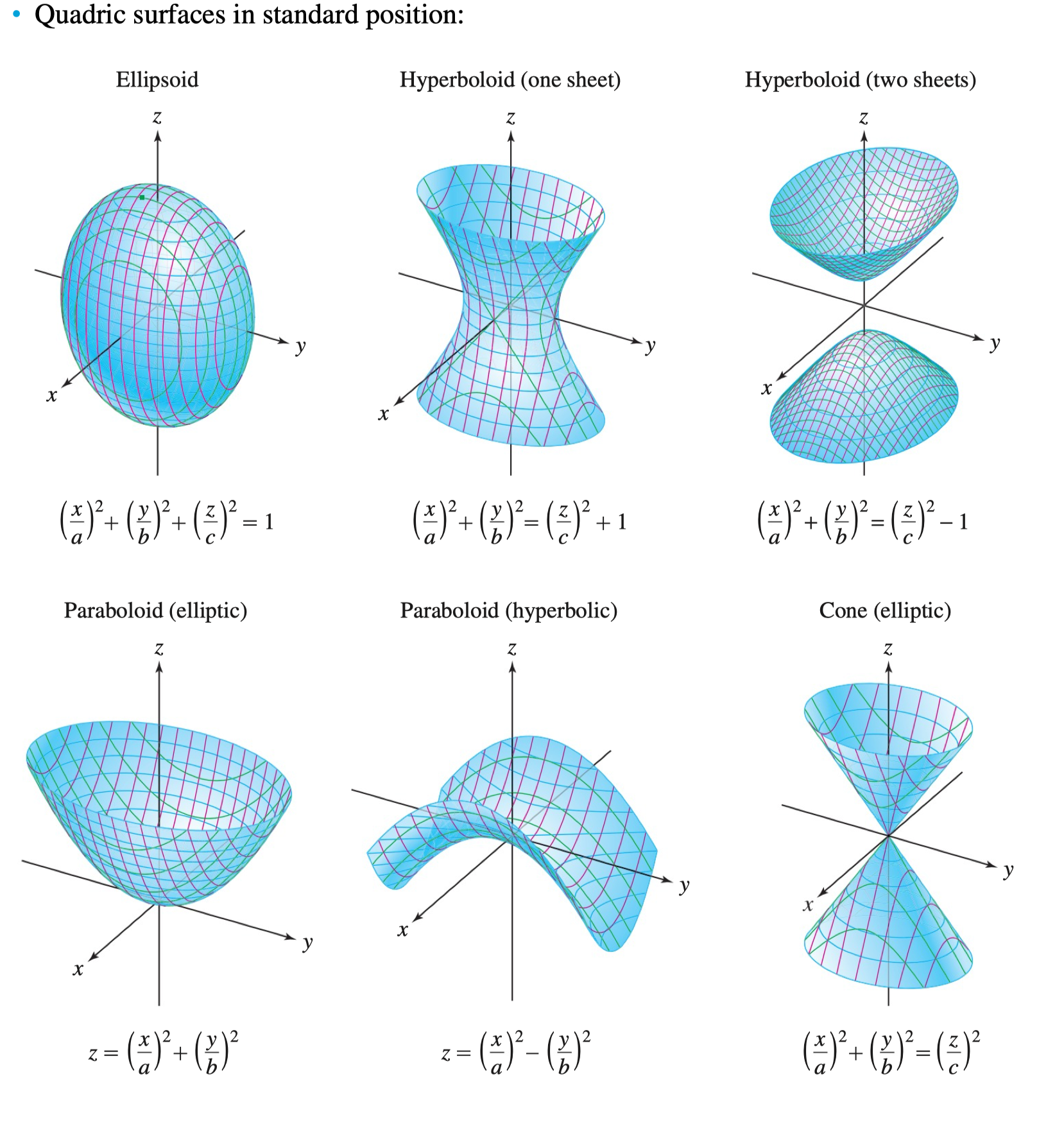
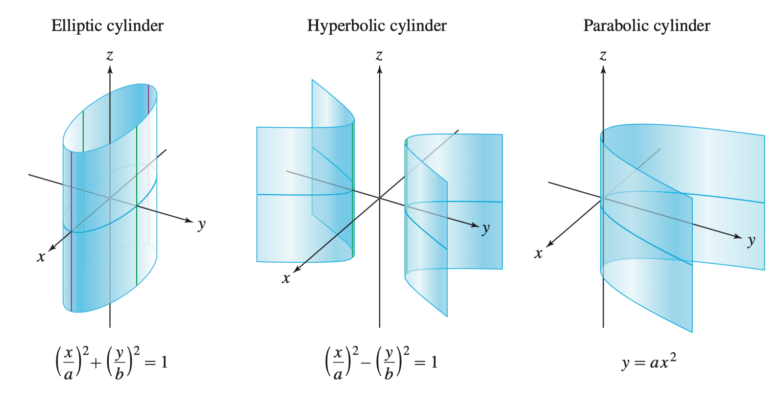
12.6 A Survey of Quadric Surfaces 二次曲面

\[ A x^{2} + B y^{2} + C z^{2} + Dxy + Eyz + Fzx + ax + by + cz + d = 0 \]

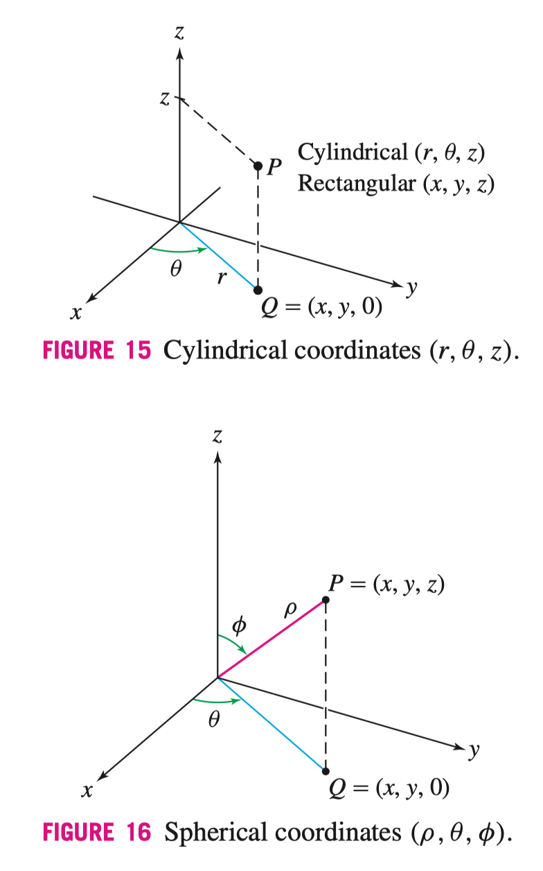
12.7 Cylindrical and Spherical Coordinates 柱面坐标系与球面坐标系

• Rectangular -> Cylindrical, Spherical

\[ \def\arraystretch{1.5} \begin{array} { c | c }\text{ Cylindrical} & \text{ Spherical } \\ \hline r^{2} = x^{2} + y^{2} & \rho^{2} = x^{2} + y^{2} + z^{2} \\ \tan(\theta) = \frac{y}{x} & \tan(\theta) \frac{y}{x} \\ z = z & \cos(\phi) = \frac{z}{\rho} \end{array} \]

其中 \(0 \leqslant \theta \leqslant 2\pi\), \(0 \leqslant \phi \leqslant \pi\)

• Cylindrical, Spherical -> Rectangular

\[ \def\arraystretch{1.5} \begin{array} { c | c }\text{ Cylindrical} & \text{ Spherical } \\ \hline x = r \cos(\theta) & x = \rho \sin(\phi) \cos(\theta) \\ y = r \sin(\theta) & y = \rho \sin(\phi) \sin(\theta) \\ z = z & z = \rho \cos(\phi) \end{array} \]

• Level Surfaces